outputDelay
Syntax
Description
D = outputDelay(sysobj)D results from the group delay of the
convolution stages within the filter.
Use this syntax when sysobj is a linear-phase single-rate filter.
To determine if a filter object has linear phase, use the islinphase
function.
[
also returns the input frequency band D,FsOut,B] = outputDelay(sysobj)B over which the delay value is
within the default tolerance of 5% (in input sample units) of D. That
is, , where f is a frequency in the band
B and FsIn is the input sample rate.
Use this syntax when sysobj has filter stages that have a nonlinear
phase.
[___] = outputDelay(
specifies options using one or more name-value arguments in addition to the input arguments
in previous syntaxes. For example,
sysobj,Name=Value)outputDelay(sysobj,
Tolerance=0.01) estimates the band of input frequencies over which
the delay value is within the tolerance of 1%.
Use this syntax to specify InputSampleRate,
CarrierFrequency, Tolerance, and
FFTLength.
Examples
Compute the output delay of a cascade of dsp.FIRRateConverter objects. Use this delay value to plot the input and resampled signals on the same plot in a time scope.
Resample Input Signal
First, let us inspect the delay and scaling that occurs in filtering. To do that, create a sinusoidal input signal. Initialize a cascade of dsp.FIRRateConverter objects to resample the input signal.
n = (0:7*17-1)';
u = cos(6*pi*n/147);
src = cascade(dsp.FIRRateConverter(13,17), dsp.FIRRateConverter(18,7))
src =
  dsp.FilterCascade with properties:

         Stage1: [1×1 dsp.FIRRateConverter]
         Stage2: [1×1 dsp.FIRRateConverter]
    CloneStages: true
Resample the input signal by passing the signal through the cascade of dsp.FIRRateConverter objects.
y = src(u);
Plot the Input and Output Signals
Initialize a time scope using the timescope object to visualize the input and the resampled signals.
tsnosync = timescope(NumInputPorts=2,...
            ChannelNames={'Input','Output'});
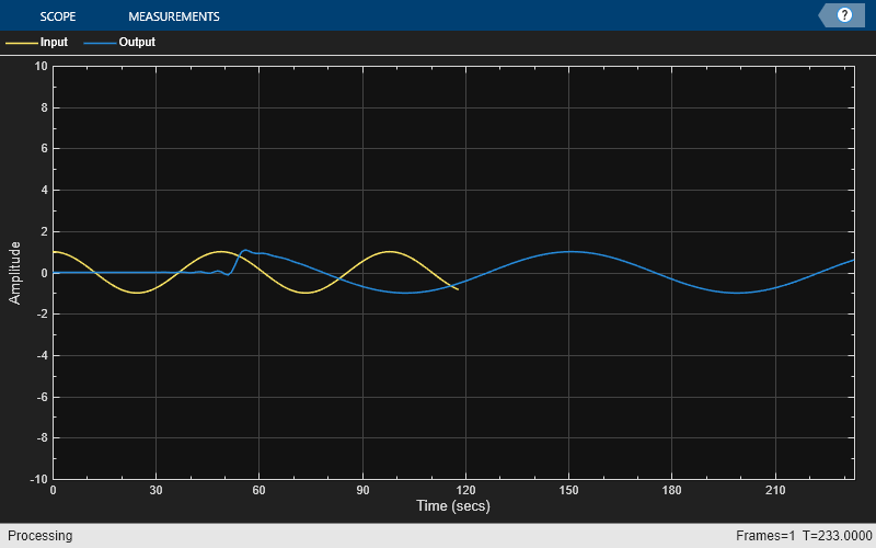
Plot the input and the resampled signals on the same plot in the time scope. You can see that the two signals are out of sync with respect to each other by a certain amount of delay and stretch over a different time scale
tsnosync(u,y);
Using outputDelay to Synchronize Signals
To plot the input and resampled signals on the same plot, you need to account for the output delay of the filter. To compute the output delay, use the outputDelay function. The value of this delay depends on the filter structure and order, the rate conversion factor, and the signal input to the filter. In addition to the output delay, the rate conversion operation of the filter introduces scaling on the time domain. You must account for the output delay and the scaling.
Use the outputDelay function to compute the delay and the output sample rate introduced by the multirate filter. You can optionally specify the input sample rate to the function. Apply the delay value to the output signal through the TimeDisplayOffset property of the time scope.
To account for the scaling, specify the input and output sample rates through the SampleRate property of the time scope. The inverse of the input and output sample rates vector determines the x-axis (time axis) spacing between points in the input signal and the output signal, respectively.
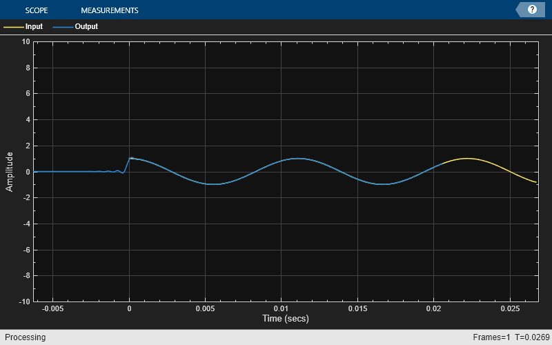
Initialize the time scope to use the updated TimeDisplayOffet and SampleRate properties. Visualize the input and the resampled signals on the time scope. With the delay and scaling accounted for, you can see that signals are synchronized and have no delay with respect to each other.
FsIn = 44.1e2;
[D,FsOut] = outputDelay(src,InputSampleRate=FsIn);

tssync = timescope(NumInputPorts=2,...
            SampleRate=[FsIn FsOut], ...
            TimeDisplayOffset=[0, -D],...
            ChannelNames={'Input','Output'});
tssync(u,y);
Compute the output delay for a farrow rate converter, and use this delay value to plot the input sinusoidal signal and the rate converted signal on the same plot.
Create an input sinusoidal signal using the sin function. Initialize the dsp.FarrowRateConverter object to model the farrow rate converter.
u = sin(6*pi*(1:50)'/200);
FsIn = 48000;
frc = dsp.FarrowRateConverter(FsIn, 44100);
Compute the output delay of the rate converter using the outputDelay function.
[D, FsOut] = outputDelay(frc)
D =
4.1667e-05
FsOut =
44100
Resample the input using the farrow rate converter. Visualize the input signal and the resampled signal on the time scope. To account for the time delay and the scaling, set the TimeDisplayOffset and SampleRate properties of the time scope to [] and [FsIn FsOut], respectively.
y = frc(u);
ts = timescope(NumInputPorts = 2, SampleRate = [FsIn FsOut], ...
    TimeDisplayOffset = [0, -D],...
    ChannelNames = {'Input','Output'}, ...
    TimeSpan = length(y)*1.1/FsIn, ...
    PlotType = 'stem');
ts(u, y);

Nonlinear phase filters have a group delay that depends on the input frequency. Due to the nonlinear phase nature, such filters distort input signals. Therefore, the output of these filters cannot be obtained by shifting and scaling the input on the time domain. To use the outputDelay function to compute the output delay of such filters, the filters must have a relatively constant group delay over the input signal band.
Start by calculating the frequency band of two nonlinear fractional delay FIR filters with partially flat group delay. One filter has a higher bandwidth compared to the other filter. Note the effect of the higher bandwidth on the output delay and the input frequency band over which the function computes the delay.
Then, consider a multirate filter cascade that has a highly nonlinear group delay response over a given band but has a relatively flat group delay over other frequency bands. Increase the tolerance value that you specify to the outputDelay function and see the effect on the input frequency band that the function returns.
Fractional Delay FIR Filter with Nonlinear Phase and Partially Flat Group Delay
Since the fractional delay FIR filter has a nonlinear phase response, specify a center frequency around which the outputDelay function should compute the delay. When you specify the center frequency, the function returns an interval of frequencies (as the third output argument) over which the delay value is within the specified tolerance.
Design a fractional delay filter using the designFracDelayFIR function. Specify the filter to have a fractional delay of 1.25e-3 seconds and a passband coverage of 50%.
FsIn = 20;
Fc = 1;
FD = 1.25e-3;

nlPhaseFilterObj1 = designFracDelayFIR(FractionalDelay=FD*FsIn,Bandwidth=0.5,SystemObject=true);
Using the outputDelay function, calculate the output delay around the center frequency of 1 Hz. Specify the input sample rate to 20 Hz and the tolerance to 0.01 (1%). In addition to the output delay, the function returns the input band over which the deviation in delay is up to 1% of D1.
[D1,~,B1] = outputDelay(nlPhaseFilterObj1,InputSampleRate=FsIn,CarrierFrequency=Fc,Tolerance=0.01)
D1 =
0.1513
B1 = 1×2

   -6.3794    6.3794
Use the grpdelay function to compute the group delay G of the filter and the frequencies W (in Hz) at which the group delay is evaluated. Specify the FFT length to 8192, and the sample rate to be the same as the input sample rate.
Plot the overall filter group delay. On the same figure, plot the input frequency band and the output delay value at the center frequency. The input frequency band indeed contains the center frequency.
[G1,W1] = grpdelay(nlPhaseFilterObj1,8192,FsIn); % Use 8192 FFT points to calculate the group delay
I1 = W1>=B1(1) & W1<=B1(2);  % Mask applicable frequencies

plot(W1,G1/FsIn);
hold on
plot(W1(I1),G1(I1)/FsIn,'r',LineWidth=2);
plot(Fc,D1,'ro');
yline(D1+0.01/FsIn*[-1 1],'k:');

title(sprintf('Applicable Band (InputSampleRate=%iHz,CarrierFrequency=%1.1fHz)',FsIn,Fc))
legend('Output delay (in sample time units)',...
    'Applicable input frequencies band',...
    'Output delay for carrier frequency',...
    'Tolerance around the nominal delay',Location='best')
ylabel('Delay (sec)')
xlabel('Frequency (Hz)')
hold off

Comparing with Higher Bandwidth Design
Compare the previous design with a higher bandwidth fractional delay design. For more information on the bandwidth of a fractional-delay FIR filter, see designFracDelayFIR.
Design a fractional-delay FIR filter with the same fractional delay (1.25e-3 seconds) as the previous design but with a 70% bandwidth coverage.
nlPhaseFilterObj2 = designFracDelayFIR(FractionalDelay=FD*FsIn,Bandwidth=0.7,SystemObject=true);
Measure the output delay of this alternative design. The output delay D2 is larger due to the longer FIR length, but the input band is also larger, allowing signals up to 7.2Hz (compared with only 6.4 Hz in the previous design).
[D2,~,B2] = outputDelay(nlPhaseFilterObj2,InputSampleRate=FsIn,CarrierFrequency=Fc,Tolerance=0.01)
D2 =
0.2512
B2 = 1×2

   -7.2217    7.2217
[G2,W2] = grpdelay(nlPhaseFilterObj2,8192,FsIn);
Plot the group delay response of the alternative design against the design with a 50% coverage.
I2 = W2>=B2(1) & W2<=B2(2);  % Mask applicable frequencies

plot(W1,G1/FsIn);
hold on
plot(W2,G2/FsIn);
plot(W1(I1),G1(I1)/FsIn,'r',LineWidth=2);
plot(W2(I2),G2(I2)/FsIn,'m',LineWidth=2);
title(sprintf('Applicable Band (InputSampleRate=%iHz,CarrierFrequency=%1.1fHz)',FsIn,Fc))
legend('Output delay (in sample time units) of design 1',...
    'Output delay (in sample time units) of design 2',...
    'Applicable input frequencies band of design 1',...
    'Applicable input frequencies band of design 2',...
    Location='best')
ylabel('Delay (sec)')
xlabel('Frequency (Hz)')
hold off

Multirate Filter Cascade with Nonlinear Phase
Design a two-stage filter cascade that contains a stable IIR lowpass (which has a nonlinear phase) followed by an FIR decimator with a rate conversion factor of 2.
FsIn = 10;
Fc = 1.5;
LP = dsp.LowpassFilter(FilterType='IIR',SampleRate=FsIn,PassbandFrequency=2.3,StopbandFrequency=2.7);
nlPhaseCascadeObj = cascade(LP,dsp.FIRDecimator(2),InputSampleRate="auto");
Measure the output delay, output sample rate, and the input frequency band for this cascade using a narrowband input signal with a carrier frequency of 1.5Hz. Set the tolerance to 0.001 samples. The function returns an output sample rate of 5 Hz (which is half the input sample rate of 10 Hz, owing to the half-rate decimator).
[D,FsOut,B] = outputDelay(nlPhaseCascadeObj,CarrierFrequency=Fc,Tolerance=0.001)
D =
2.9209
FsOut =
5
B = 1×2

    1.5000    1.5000
The band the function returns is a trivial band. That is, it contains a single point (the left and right boundaries are the same). This means that a tolerance value of 0.001 is too small.
To fix that, increase the tolerance to 0.05 seconds (0.5 of the input sample time). While the delay and the output sample rate do not change, the band is now nontrivial, and it contains the center frequency. The band is also relatively narrow due to the highly nonlinear phase nature of the IIR design.
[D1,FsOut1,B1] = outputDelay(nlPhaseCascadeObj,CarrierFrequency=Fc,Tolerance=0.5)
D1 =
2.9209
FsOut1 =
5
B1 = 1×2

    1.3562    1.5967
Increase the tolerance value to 2. The band now increases even more as you have specified a more lax tolerance.
[D2,FsOut2,B2] = outputDelay(nlPhaseCascadeObj,CarrierFrequency=Fc,Tolerance=2)
D2 =
2.9209
FsOut2 =
5
B2 = 1×2

    0.4565    1.7786
[G,W] = grpdelay(nlPhaseCascadeObj,8192,FsIn);
I1 = W>=B1(1) & W<=B1(2);  % Mask applicable frequencies
I2 = W>=B2(1) & W<=B2(2);  % Mask applicable frequencies

plot(W,G/FsIn);
hold on
plot(W(I2),G(I2)/FsIn,Color=[0.6 0.1 0.6],LineWidth=2);
plot(W(I1),G(I1)/FsIn,Color=[0 0.7 0.7],LineWidth=4);
plot(Fc,D1,'ro');
title(sprintf('Applicable Band (InputSampleRate=%iHz,CarrierFrequency=%1.1fHz)',FsIn,Fc))
legend('Output delay (in sample time units)',...
    'Applicable input frequencies band with Tolerance=1',...
    'Applicable input frequencies band with Tolerance=0.5',...
    'Output delay for carrier frequency',...
    Location='best')
ylabel('Delay (sec)')
xlabel('Frequency (Hz)')
hold off

Input Arguments
Name-Value Arguments
Output Arguments
More About
A multirate filter is any cascade combining upsampling, downsampling, and convolution filters (FIR or IIR).
![]()
Most filter System objects in DSP System Toolbox™ are multirate filters. For example, dsp.FIRDecimator(5) is
the multirate filter H(z) followed by a downsampler
that has a downsampling ratio of 5.
Single-rate filters are special
cases of multirate filters with
a rate conversion factor of 1. Single-stage filters are special cases of cascades of
multirate filters. For example, dsp.LowpassFilter is a single-rate,
single-stage filter of the form H(z).
The outputDelay function assumes that the multirate filter
sysobj models a resampling system. The output of the resampling
system is a filtered and resampled version of the input, and hence has a different rate
compared to the input.
A resampling system interpolates the input u(n) to a continuous domain function f(t) that approximates the input.
The output is then sampled from f(t) on a different time scale.
The values FsIn and FsOut are
the input and output sample rates, respectively, and D is the
resampling or output delay.
This graph overlays the input and output sequences on the same plot, shows the input and output sample times, and also shows the output delay that the function returns.

For examples that demonstrate the effect of the resampling delay and scaling in multirate filters, see Compute Output Delay of Filter Cascade and Time Delay and Scaling in Multirate DSP Filters.
The output delay and the group delay are related to each other.
The output or resampling delay is the delay of the signal in time units as it goes
through a convolution filter (FIR or IIR). For a single-rate filter, the output delay
(D) and the group delay () are scaled by the sample rate, . If the filter has a linear phase, both the output delay and the group
delay do not depend on the input frequency. However, if the filter has nonlinear phase, then
the group delay and the output delay depend on the input frequency.
This figure shows the impulse response of a symmetric 24-tap FIR filter. You can see that the output delay and the group delay are equivalent quantities in different scales.

If the filter is a multirate filter, the output delay is the total delay that the filter
accumulates on all stages of the cascade. The output sample rate FsOut
of each stage becomes the input sample rate FsIn of the subsequent
stage. The function scales the delay values accumulated over each stage by the rate
conversion factors of the individual stages.
The group delay is defined only for single-rate filters while the output delay is defined for both single-rate and multirate filters.
The group delay refers to the average delay of the convolution filter (FIR or IIR) as a function of frequency. It is computed as the negative first derivative of the phase response of the filter. If the frequency response of a filter is H(ejω), then the group delay is
where θ(ω) is the phase, or argument, of H(ejω).
If the filter is a linear phase filter, the group delay response is flat. The output
delay D does not depend on input frequency. If the filter is a
nonlinear phase filter, the group delay response varies with frequency and the delay value
D is valid only for bandlimited inputs around a carrier frequency
Fc. The function determines the edges of the frequency band
B such that the group delay over this frequency region is
approximately constant. For more information, see Linear and Nonlinear Phase Filters. For an example, see Time Delay and Scaling in Multirate DSP Filters.
Consider the multirate filter cascade below with nonlinear phase filter stages Q(z) and R(z).

The noble identify for decimation is given by:
![]()
Apply the noble identity for decimation on R(z). The product Q(z)R(z2) is a linear phase system.

Even though the individual filter stages have a nonlinear phase, the combined equivalent
filter after applying the noble identify has a linear phase. The
outputDelay function treats this filter as a linear phase
filter.
All combinations of nonlinear phase stages cannot be reordered to form linear phase equivalents. The function treats such filters as nonlinear filters and operates in the bandlimited mode.