forecast
Forecast states and observations of diffuse state-space models
Syntax
Description
[ returns forecasted observations (Y,YMSE]
= forecast(Mdl,numPeriods,Y0)Y)
and their corresponding variances (YMSE) from forecasting
the diffuse
state-space model Mdl using a numPeriods forecast
horizon and in-sample observations Y0.
[ uses
additional options specified by one or more Y,YMSE]
= forecast(Mdl,numPeriods,Y0,Name,Value)Name,Value pair
arguments. For example, for state-space models that include a linear
regression component in the observation model, include in-sample predictor
data, predictor data for the forecast horizon, and the regression
coefficient.
Input Arguments
Name-Value Arguments
Output Arguments
Examples
Suppose that a latent process is a random walk. The state equation is
where is Gaussian with mean 0 and standard deviation 1.
Generate a random series of 100 observations from , assuming that the series starts at 1.5.
T = 100;
x0 = 1.5;
rng(1); % For reproducibility
u = randn(T,1);
x = cumsum([x0;u]);
x = x(2:end);
Suppose further that the latent process is subject to additive measurement error. The observation equation is
where is Gaussian with mean 0 and standard deviation 0.75. Together, the latent process and observation equations compose a state-space model.
Use the random latent state process (x) and the observation equation to generate observations.
y = x + 0.75*randn(T,1);
Specify the four coefficient matrices.
A = 1;
B = 1;
C = 1;
D = 0.75;
Create the diffuse state-space model using the coefficient matrices. Specify that the initial state distribution is diffuse.
Mdl = dssm(A,B,C,D,'StateType',2)Mdl =
State-space model type: dssm
State vector length: 1
Observation vector length: 1
State disturbance vector length: 1
Observation innovation vector length: 1
Sample size supported by model: Unlimited
State variables: x1, x2,...
State disturbances: u1, u2,...
Observation series: y1, y2,...
Observation innovations: e1, e2,...
State equation:
x1(t) = x1(t-1) + u1(t)
Observation equation:
y1(t) = x1(t) + (0.75)e1(t)
Initial state distribution:
Initial state means
x1
0
Initial state covariance matrix
x1
x1 Inf
State types
x1
Diffuse
Mdl is an dssm model. Verify that the model is correctly specified using the display in the Command Window.
Forecast observations 10 periods into the future, and estimate the mean squared errors of the forecasts.
numPeriods = 10;
[ForecastedY,YMSE] = forecast(Mdl,numPeriods,y);
Plot the forecasts with the in-sample responses, and 95% Wald-type forecast intervals.
ForecastIntervals(:,1) = ForecastedY - 1.96*sqrt(YMSE);
ForecastIntervals(:,2) = ForecastedY + 1.96*sqrt(YMSE);

figure
plot(T-20:T,y(T-20:T),'-k',T+1:T+numPeriods,ForecastedY,'-.r',...
    T+1:T+numPeriods,ForecastIntervals,'-.b',...
    T:T+1,[y(end)*ones(3,1),[ForecastedY(1);ForecastIntervals(1,:)']],':k',...
    'LineWidth',2)
hold on
title({'Observed Responses and Their Forecasts'})
xlabel('Period')
ylabel('Responses')
legend({'Observations','Forecasted observations','95% forecast intervals'},...
    'Location','Best')
hold off
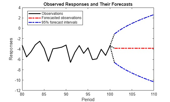
The forecast intervals flare out because the process is nonstationary.
Suppose that the linear relationship between unemployment rate and the nominal gross national product (nGNP) is of interest. Suppose further that unemployment rate is an AR(1) series. Symbolically, and in state-space form, the model is
where:
is the unemployment rate at time t.
is the observed change in the unemployment rate being deflated by the return of nGNP ().
is the Gaussian series of state disturbances having mean 0 and unknown standard deviation .
Load the Nelson-Plosser data set, which contains the unemployment rate and nGNP series, among other things.
load Data_NelsonPlosserPreprocess the data by taking the natural logarithm of the nGNP series and removing the starting NaN values from each series.
isNaN = any(ismissing(DataTable),2);       % Flag periods containing NaNs
gnpn = DataTable.GNPN(~isNaN);
y = diff(DataTable.UR(~isNaN));
T = size(gnpn,1);                          % The sample size
Z = price2ret(gnpn);
This example continues using the series without NaN values. However, using the Kalman filter framework, the software can accommodate series containing missing values.
Determine how well the model forecasts observations by removing the last 10 observations for comparison.
numPeriods = 10;                   % Forecast horizon
isY = y(1:end-numPeriods);         % In-sample observations
oosY = y(end-numPeriods+1:end);    % Out-of-sample observations
ISZ = Z(1:end-numPeriods);         % In-sample predictors
OOSZ = Z(end-numPeriods+1:end);  % Out-of-sample predictors
Specify the coefficient matrices.
A = NaN;
B = NaN;
C = 1;
Create the state-space model using dssm by supplying the coefficient matrices and specifying that the state values come from a diffuse distribution. The diffuse specification indicates complete ignorance about the moments of the initial distribution.
StateType = 2;
Mdl = dssm(A,B,C,'StateType',StateType);
Estimate the parameters. Specify the regression component and its initial value for optimization using the 'Predictors' and 'Beta0' name-value pair arguments, respectively. Display the estimates and all optimization diagnostic information. Restrict the estimate of to all positive, real numbers.
params0 = [0.3 0.2]; % Initial values chosen arbitrarily
Beta0 = 0.1;
[EstMdl,estParams] = estimate(Mdl,y,params0,'Predictors',Z,'Beta0',Beta0,...
    'lb',[-Inf 0 -Inf]);
Method: Maximum likelihood (fmincon)
Effective Sample size:             60
Logarithmic  likelihood:     -110.477
Akaike   info criterion:      226.954
Bayesian info criterion:      233.287
           |      Coeff       Std Err    t Stat    Prob
--------------------------------------------------------
 c(1)      |   0.59436       0.09408     6.31738  0
 c(2)      |   1.52554       0.10758    14.17991  0
 y <- z(1) | -24.26161       1.55730   -15.57930  0
           |
           |    Final State   Std Dev     t Stat   Prob
 x(1)      |   2.54764        0           Inf     0
EstMdl is a dssm model, and you can access its properties using dot notation.
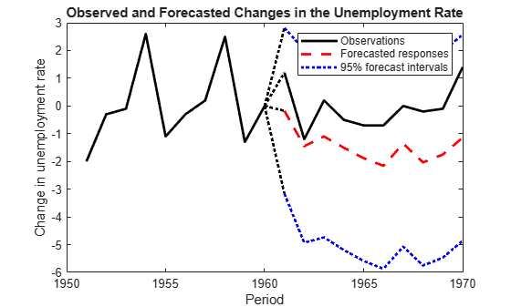
Forecast observations over the forecast horizon. EstMdl does not store the data set, so you must pass it in appropriate name-value pair arguments.
[fY,yMSE] = forecast(EstMdl,numPeriods,isY,'Predictors0',ISZ,...
    'PredictorsF',OOSZ,'Beta',estParams(end));
fY is a 10-by-1 vector containing the forecasted observations, and yMSE is a 10-by-1 vector containing the variances of the forecasted observations.
Obtain 95% Wald-type forecast intervals. Plot the forecasted observations with their true values and the forecast intervals.
ForecastIntervals(:,1) = fY - 1.96*sqrt(yMSE);
ForecastIntervals(:,2) = fY + 1.96*sqrt(yMSE);

figure
h = plot(dates(end-numPeriods-9:end-numPeriods),isY(end-9:end),'-k',...
    dates(end-numPeriods+1:end),oosY,'-k',...
    dates(end-numPeriods+1:end),fY,'--r',...
    dates(end-numPeriods+1:end),ForecastIntervals,':b',...
    dates(end-numPeriods:end-numPeriods+1),...
    [isY(end)*ones(4,1),[oosY(1);ForecastIntervals(1,:)';fY(1)]],':k',...
    'LineWidth',2);
xlabel('Period')
ylabel('Change in unemployment rate')
legend(h([1,3,4]),{'Observations','Forecasted responses',...
    '95% forecast intervals'})
title('Observed and Forecasted Changes in the Unemployment Rate')
Suppose that a latent process is a random walk. The state equation is
where is Gaussian with mean 0 and standard deviation 1.
Generate a random series of 100 observations from , assuming that the series starts at 1.5.
T = 100;
x0 = 1.5;
rng(1); % For reproducibility
u = randn(T,1);
x = cumsum([x0;u]);
x = x(2:end);
Suppose further that the latent process is subject to additive measurement error. The observation equation is
where is Gaussian with mean 0 and standard deviation 0.75. Together, the latent process and observation equations compose a state-space model.
Use the random latent state process (x) and the observation equation to generate observations.
y = x + 0.75*randn(T,1);
Specify the four coefficient matrices.
A = 1;
B = 1;
C = 1;
D = 0.75;
Create the diffuse state-space model using the coefficient matrices. Specify that the initial state distribution is diffuse.
Mdl = dssm(A,B,C,D,'StateType',2)Mdl =
State-space model type: dssm
State vector length: 1
Observation vector length: 1
State disturbance vector length: 1
Observation innovation vector length: 1
Sample size supported by model: Unlimited
State variables: x1, x2,...
State disturbances: u1, u2,...
Observation series: y1, y2,...
Observation innovations: e1, e2,...
State equation:
x1(t) = x1(t-1) + u1(t)
Observation equation:
y1(t) = x1(t) + (0.75)e1(t)
Initial state distribution:
Initial state means
x1
0
Initial state covariance matrix
x1
x1 Inf
State types
x1
Diffuse
Mdl is an dssm model. Verify that the model is correctly specified using the display in the Command Window.
Forecast states 10 periods into the future, and estimate the mean squared errors of the forecasts.
numPeriods = 10;
[~,~,ForecastedX,XMSE] = forecast(Mdl,numPeriods,y);
Plot the forecasts with the in-sample states, and 95% Wald-type forecast intervals.
ForecastIntervals(:,1) = ForecastedX - 1.96*sqrt(XMSE);
ForecastIntervals(:,2) = ForecastedX + 1.96*sqrt(XMSE);

figure
plot(T-20:T,x(T-20:T),'-k',T+1:T+numPeriods,ForecastedX,'-.r',...
    T+1:T+numPeriods,ForecastIntervals,'-.b',...
    T:T+1,[x(end)*ones(3,1),[ForecastedX(1);ForecastIntervals(1,:)']],':k',...
    'LineWidth',2)
hold on
title({'State Values and Their Forecasts'})
xlabel('Period')
ylabel('State value')
legend({'State Values','Forecasted states','95% forecast intervals'},...
    'Location','Best')
hold off
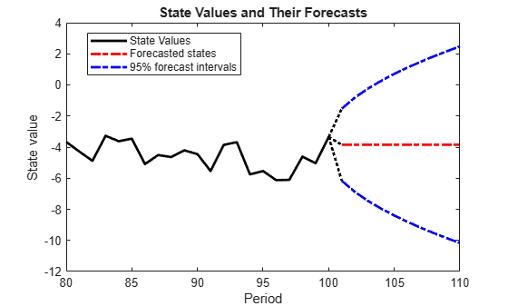
The forecast intervals flare out because the process is nonstationary.
Tips
Mdl does not store the response data, predictor
data, and the regression coefficients. Supply them whenever necessary
using the appropriate input or name-value pair arguments.
Algorithms
The Kalman filter accommodates missing data by not updating filtered state estimates corresponding to missing observations. In other words, suppose there is a missing observation at period t. Then, the state forecast for period t based on the previous t – 1 observations and filtered state for period t are equivalent.
References
[1] Durbin J., and S. J. Koopman. Time Series Analysis by State Space Methods. 2nd ed. Oxford: Oxford University Press, 2012.
Version History
Introduced in R2015b