Estimate Threshold-Switching Dynamic Regression Models

This example shows how to use the estimate function to fit threshold-switching dynamic regression models to simulated data and to tune the estimation procedure. The example estimates a self-exciting threshold autoregressive model (SETAR), a TAR model with an exogenous threshold variable, and a self-exciting smooth TAR model (SESTAR) containing a regression component.

Threshold-switching dynamic regression model estimation, performed by estimate, is an iterative two-step procedure:

1. Conduct a constrained, nonlinear search over threshold transition levels and rates.

2. Solve a linear least-squares problem for submodel parameters.

The resulting estimates of parameter standard errors, data loglikelihood, and model residuals are conditional on the optimal threshold parameters computed by the search.

Simulate Data from SETAR DGP

Consider a data-generating process (DGP) for the following simple univariate, mean-switching, SETAR model:

• The discrete, endogenous threshold transition is at mid-level 1.5.

• ${\sigma }^2=1$ is the model-wide process variance.

• The state 1 submodel is ${\mathit{y}}_{1,\mathit{t}}=0.2{\mathit{y}}_{1,\mathit{t}-1}+{\epsilon }_{1.\mathit{t}}$, where ${\epsilon }_{1,\mathit{t}}\sim {\rm N}\left(0,{\sigma }^2\right)$.

• The state 2 submodel is ${\mathit{y}}_{2,\mathit{t}}=0.4{\mathit{y}}_{2,\mathit{t}-1}+{\epsilon }_{2.\mathit{t}}$, where ${\epsilon }_{2,\mathit{t}}\sim {\rm N}\left(0,{\sigma }^2\right)$.

Create a SETAR model that represents the DGP by following this procedure:

1. Create the threshold transition by using the threshold function. The resulting threshold object represents all aspects of the threshold transition except for whether the associated threshold variable is endogenous or exogenous to the threshold-switching model system.

2. Create each univariate submodel by using the arima function. The resulting arima objects each characterize the dynamics of the system within their respective states. Concatenate the model objects in a vector.

3. Create the threshold-switching model by passing the threshold transitions object and state submodel vector to the tsVAR function. Specify the model-wide covariance by using the Covariance name-value argument. The resulting tsVAR object represents all aspects of the threshold-switching model for whether the associated threshold variable is endogenous or exogenous to its system. Object functions of the tsVAR object require knowledge of the threshold variable type (the default is endogenous or self-exciting for all object functions, with a delay of 1 time step).

midlvl = 1.5;
ttDGP = threshold(midlvl);

mdl1DGP = arima(Constant=0,AR=0.2);
mdl2DGP = arima(Constant=2,AR=0.4);
MdlDGP = tsVAR(ttDGP,[mdl1DGP mdl2DGP],Covariance=1);

MdlDGP is a tsVAR object that represents the DGP. It is fully specified because all parameters are set to known values.

Generate a random path of length 500 from the SETAR DGP by using the simulate object function. Plot the threshold transition and the path.

seed = 0;
rng(seed)               % For reproducibility
T = 500;                % Sample size
Y = simulate(MdlDGP,T); % SETAR path

figure
ttplot(ttDGP,Data=Y)

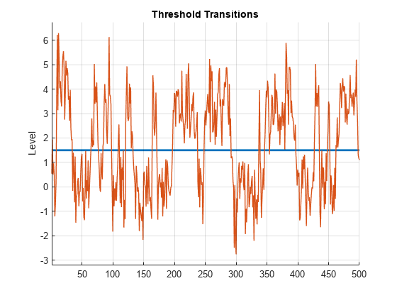
The plot shows the self-exciting response variable sampling states on either side of the threshold level. In practice, without knowledge of the DGP, a plot of empirical data in Y informs a reasonable choice of the initial threshold level, which is estimate requires.

Create Model Template for Estimation

To estimate a SETAR model of the data, create the following variables:

• A model template for estimation, which is a partially specified tsVAR object that indicates the structure of the target model with NaN values for estimable parameters

• A threshold transition to initialize the search, which is a fully specified threshold object. This example uses 1 as the initial mid-level.

tt = threshold(NaN);
mdl1 = arima(Constant=NaN,AR=NaN);
mdl2 = arima(Constant=NaN,AR=NaN);
Mdl = tsVAR(tt,[mdl1 mdl2],Covariance=NaN);

t0 = 1; % Initial mid-level
tt0 = threshold(t0,Type="discrete");

Fit SETAR Model to Data

Discrete transitions pose a unique estimation challenge because they fail to disambiguate levels that fall between threshold variable data, which produces discontinuous objective functions that are difficult to optimize. To address this problem, estimate treats discrete transition levels as high-rate logistic transitions before it converts to discrete levels and discards the rates at estimation termination [1]. The MaxRate name-value argument specifies the upper bound for the rates estimate uses for estimation.

This code shows the internal representation of the discrete transition during estimation by plotting a logistic threshold transition at mid-level 1.5 with rate 10.

maxRate = 10;
ttEst = threshold(midlvl,Type="logistic",Rates=maxRate);

figure
ttplot(ttEst,Data=Y)
colorbar("off")

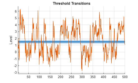
The logistic transition combines the two submodels in a weighted mixture model that is responsive to continuous changes in level during the threshold search procedure. estimate automatically implements the transformation from a discrete to a logistic representation at the beginning of estimation, and then it reverse-transforms the resulting threshold transition at estimation termination.

Estimate the SETAR model by passing the model template Mdl, initial threshold transition tt0, and simulated path Y to estimate. Set the maximum transition rate to 10. By default, the threshold variable is endogenous (Type="endogenous") with a delay of one time step (Delay=1).

EstMdl = estimate(Mdl,tt0,Y,MaxRate=maxRate);

EstMdl is a fully specified tsVAR object representing the estimated SETAR model with a discrete threshold transition. estimate uses the maximum rate maxRate only internally because it represents the discrete transition as logistic to overcome numerical problems during optimization. To tune the estimation procedure for any threshold transition type, you can iterate by adjusting MaxRate and calling estimate.

Inspect Estimation Results

Display the estimated threshold transition Switch, stored in the estimated model object, by using dot notation.

EstTT = EstMdl.Switch

EstTT = 
  threshold with properties:

          Type: 'discrete'
        Levels: 1.5233
         Rates: []
    StateNames: ["1"    "2"]
     NumStates: 2

Display the estimated submodels.

EstMdl.Submodels

ans = 
  2×1 varm array with properties:

    NumSeries
    P
    Constant
    AR
    Beta
    Trend
    Covariance
    SeriesNames
    Description

Observe that estimate returns a vector of varm model objects representing the estimated univariate models, although the model template Mdl specifies a vector of arima model objects.

Visually compare the estimated parameters to those of the DGP.

EstMdlParams = [EstMdl.Switch.Levels; ...
           EstMdl.Submodels(1).Constant; ...
           EstMdl.Submodels(2).Constant; ...
           EstMdl.Submodels(1).AR{:}; ...
           EstMdl.Submodels(2).AR{:}; ...
           EstMdl.Covariance];

DGPParams = [MdlDGP.Switch.Levels; ...
           MdlDGP.Submodels(1).Constant; ...
           MdlDGP.Submodels(2).Constant; ...
           MdlDGP.Submodels(1).AR{:}; ...
           MdlDGP.Submodels(2).AR{:}; ...
           MdlDGP.Covariance];

table(DGPParams,EstMdlParams)

ans=6×2 table
    DGPParams    EstMdlParams
    _________    ____________

       1.5           1.5233  
         0         0.034171  
         2           1.8688  
       0.2          0.14564  
       0.4          0.41827  
         1           1.0406  

The estimation results, with sufficient sample size and a limited number of parameters, approximate values of the DGP.

Summarize the estimation results.

summarize(EstMdl)

Description
1-Dimensional tsVAR Model with 2 Submodels

Switch
Transition Type: discrete
Estimated Levels: 1.523

Fit
Effective Sample Size: 499 
Number of Estimated Parameters: 4 
Number of Constrained Parameters: 0 
LogLikelihood: -717.972 
AIC: 1443.945 
BIC: 1460.795 

Submodels
                           Estimate    StandardError    TStatistic      PValue  
                           ________    _____________    __________    __________

    State 1 Constant(1)    0.034171      0.067052        0.50963         0.61031
    State 1 AR{1}(1,1)      0.14564      0.077043         1.8904          0.0587
    State 2 Constant(1)      1.8688       0.22499         8.3063      9.8696e-17
    State 2 AR{1}(1,1)      0.41827      0.064622         6.4726      9.6348e-11

Fit TAR Model with Exogenous Threshold Variable

The estimation of AR parameters in a self-exciting model is complicated by the mixed endogenous dynamics.

Compare SETAR model estimation to estimation of a TAR model, with the same general structure as the SETAR model, but with an exogenous threshold variable. Consider the threshold variable ${\mathit{z}}_{\mathit{t}}=1.5+5{\mathit{u}}_{\mathit{t}}$, where ${\mathit{u}}_{\mathit{t}}$ is standard Gaussian noise.

Simulate a random path of threshold variable observations, and then plot the threshold transition with the exogenous threshold data.

z = 1.5 + 5*randn(T,1); % Path of exogenous threshold data

figure
ttplot(ttDGP,Data=z)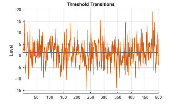

As expected, ${\mathit{z}}_{\mathit{t}}$ randomly fluctuates around the threshold.

Simulate a response path from the DGP of the TAR model. Specify that the threshold variable is exogenous and specify the simulated threshold data.

rng(seed)
Y = simulate(MdlDGP,T,Type="exogenous",Z=z);    % TAR path

Estimate the TAR model with an exogenous threshold variable. Threshold variable aside, the structure of the SETAR and TAR models are identical. Therefore, specify the SETAR model template and initial threshold transition. Specify that the threshold variable is exogenous and specify the simulated threshold data and the maximum transition rate maxRate.

EstMdlExo = estimate(Mdl,tt0,Y,MaxRate=maxRate, ...
    Type="exogenous",Z=z);

Visually compare the estimated parameters to those of the DGP.

EstMdlExoParams = [EstMdlExo.Switch.Levels; ...
           EstMdlExo.Submodels(1).Constant; ...
           EstMdlExo.Submodels(2).Constant; ...
           EstMdlExo.Submodels(1).AR{:}; ...
           EstMdlExo.Submodels(2).AR{:}; ...
           EstMdlExo.Covariance];

table(DGPParams,EstMdlParams,EstMdlExoParams)

ans=6×3 table
    DGPParams    EstMdlParams    EstMdlExoParams
    _________    ____________    _______________

       1.5           1.5233            1.5391   
         0         0.034171         0.0048078   
         2           1.8688            1.9463   
       0.2          0.14564           0.18852   
       0.4          0.41827           0.41886   
         1           1.0406            1.0216   

Overall, the estimates improve with the exogenous threshold data.

Summarize the estimation results.

summarize(EstMdlExo)

Description
1-Dimensional tsVAR Model with 2 Submodels

Switch
Transition Type: discrete
Estimated Levels: 1.539

Fit
Effective Sample Size: 499 
Number of Estimated Parameters: 4 
Number of Constrained Parameters: 0 
LogLikelihood: -713.386 
AIC: 1434.773 
BIC: 1451.623 

Submodels
                           Estimate     StandardError    TStatistic      PValue   
                           _________    _____________    __________    ___________

    State 1 Constant(1)    0.0048078       0.08187        0.058726         0.95317
    State 1 AR{1}(1,1)       0.18852      0.039812          4.7352      2.1887e-06
    State 2 Constant(1)       1.9463      0.087457          22.254     1.0253e-109
    State 2 AR{1}(1,1)       0.41886      0.040425          10.361      3.7112e-25

Tune Estimation Procedure

The MaxLevel and MaxRate name-value arguments set inequality constraints on the threshold parameter search. Estimate the TAR model with an exogenous threshold variable again. Expand the search domain by increasing the upper bound of the rate.

maxRate = 50;
EstMdlExo2 = estimate(Mdl,tt0,Y,MaxRate=maxRate,Type="exogenous",Z=z);

Compare the results of the two MaxRate settings for the TAR model esimtation.

EstMdlExoParams2 = [EstMdlExo2.Switch.Levels; ...
                 EstMdlExo2.Submodels(1).Constant; ...
                 EstMdlExo2.Submodels(2).Constant; ...
                 EstMdlExo2.Submodels(1).AR{:}; ...
                 EstMdlExo2.Submodels(2).AR{:}; ...
                 EstMdlExo2.Covariance];

table(DGPParams,EstMdlParams,EstMdlExoParams2)

ans=6×3 table
    DGPParams    EstMdlParams    EstMdlExoParams2
    _________    ____________    ________________

       1.5           1.5233            1.5185    
         0         0.034171         0.0066017    
         2           1.8688            1.9409    
       0.2          0.14564           0.18838    
       0.4          0.41827           0.41627    
         1           1.0406            1.0063    

In this case, the expanded search domain results in more accurate estimates.

Fit SESTAR Model Containing Regression Component

Accurate estimation is more challenging when the number of series, thresholds, and submodels increases for the following reasons:

• The estimates are asymptotic.

• When the estimation procedure estimates submodel parameters, the demand on the sample size increases because the procedure divides the sample into subsamples through transition-function weighting.

Consider a DGP for a bivariate, two-state, self-exciting, smooth TAR model (SESTAR) with both endogenous and exogenous dynamics:

• The smooth, normal threshold transition is at mid-level 2.5 with a transition rate of 5.

• The state 1 submodel is ${\mathit{y}}_{1,\mathit{t}}=\left[\begin{array}{c}1\\ -1\end{array}\right]+\left[\begin{array}{cc}0.5& 0\\ 0& 0.5\end{array}\right]{\mathit{y}}_{1,\mathit{t}-1}+\left[\begin{array}{c}0.3\\ -0.3\end{array}\right]{\mathit{x}}_{1,\mathit{t}}+{\epsilon }_{1.\mathit{t}}$.

• The state 2 submodel is ${\mathit{y}}_{2,\mathit{t}}=\left[\begin{array}{c}2\\ -2\end{array}\right]+\left[\begin{array}{cc}0.3& 0\\ 0& 0.3\end{array}\right]{\mathit{y}}_{2,\mathit{t}-1}+\left[\begin{array}{cc}0.4& 0\\ 0& 0.4\end{array}\right]{\mathit{y}}_{2,\mathit{t}-2}+\left[\begin{array}{cc}0.5& 0.2\\ -0.5& -0.2\end{array}\right]\left[\begin{array}{c}{\mathit{x}}_{1,\mathit{t}}\\ {\mathit{x}}_{2,\mathit{t}}\end{array}\right]+{\epsilon }_{2.\mathit{t}}$.

• ${\mathit{x}}_{1,\mathit{t}}$ and ${\mathit{x}}_{2,\mathit{t}}$ are univariate, standard Gaussian exogenous series.

• ${\epsilon }_{1,\mathit{t}}\sim {{\rm N}}_2\left(\left[\begin{array}{c}0\\ 0\end{array}\right],\left[\begin{array}{cc}1& 0\\ 0& 1\end{array}\right]\right)$ and ${\epsilon }_{2.\mathit{t}}={\epsilon }_{1,\mathit{t}}\sqrt{2}$.

Create a SETAR model that represents the DGP by following this procedure. Use varm to specify the submodel dynamics.

ttDGP = threshold(2.5,Type="normal",Rates=5);

% Constants (numSeries x 1 vectors)
c1 = [1;-1];
c2 = [2;-2];

% AR coefficients (numSeries x numSeries matrices)
AR1 = {[0.5 0; 0 0.5]};                % 1 lag
AR2 = {[0.3 0; 0 0.3] [0.4 0; 0 0.4]}; % 2 lags

% Regression coefficients (numSeries x numRegressors matrices)
beta1 = [0.3; -0.3];          % 1 regressor
Beta2 = [0.5 0.2; -0.5 -0.2]; % 2 regressors

% Innovations covariances (numSeries x numSeries matrices)
Sigma1 = [1 0; 0 1];
Sigma2 = [2 0; 0 2];

mdl1DGP = varm(Constant=c1,AR=AR1,Beta=beta1,Covariance=Sigma1);
mdl2DGP = varm(Constant=c2,AR=AR2,Beta=Beta2,Covariance=Sigma2);
MdlDGP = tsVAR(ttDGP,[mdl1DGP mdl2DGP]);

Simulate a 2-D path of standard Gaussian values for the regression data, and then simulate a 2-D response path from the DGP. By default, tsVAR object functions set the threshold variable of a multivariate self-exciting model to the first variable (Index=1).

rng(seed) 
X = rand(T,2);              % Regression data
Y = simulate(MdlDGP,T,X=X); % SESTAR path

figure
ttplot(ttDGP,Data=Y(:,1))   % Self-exciting component of Y
colorbar('off')

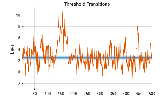
The plot indicates that the self-exciting first component of the response samples states on either side of the threshold level.

Unconstrained Estimation

Estimate the two threshold parameters and all 22 constant, AR, and regression submodel parameters from the simulated sample. To show the progress of the search procedure, create an iteration plot by using the IterationPlot name-value argument.

tt = threshold(NaN,Type="normal",Rates=NaN);
mdl1 = varm(Constant=NaN(2,1),AR={NaN(2)},Beta=NaN(2,1));
mdl2 = varm(Constant=NaN(2,1),AR={NaN(2) NaN(2)},Beta=NaN(2,2));
Mdl = tsVAR(tt,[mdl1 mdl2]);

figure
tt0 = threshold(1,Type="normal",Rates=1);
EstMdlSESTAR = estimate(Mdl,tt0,Y,X=X,IterationPlot=true);

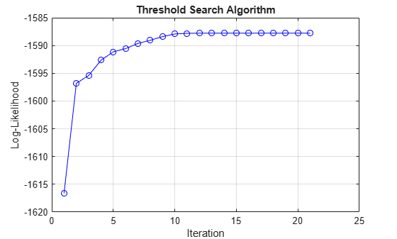
The plot indicates convergence after 20 iterations.

Compare the DGP parameters and estimated values.

compareEstimates(MdlDGP,EstMdlSESTAR)

Threshold parameters:
    2.5000    2.6484
    5.0000    4.6065



Submodel constants:
    1.0000    1.4785
   -1.0000   -1.2181
    2.0000    1.0724
   -2.0000   -1.7798



Submodel(1) AR coefficients:
    0.5000         0    0.4550    0.0710
         0    0.5000    0.0482    0.4903



Submodel(2) AR coefficients:
    0.3000         0    0.3327   -0.1410
         0    0.3000   -0.1514    0.2909
    0.4000         0    0.3539    0.4015
         0    0.4000    0.5119    0.3694



Submodel(1) regression coefficients:
    0.3000   -0.0039
   -0.3000   -0.0400



Submodel(2) regression coefficients:
    0.5000    0.2000    0.3600    0.2931
   -0.5000   -0.2000   -0.4952    0.2515



Innovations covariances:
    1.0000         0    1.1646    0.0744
         0    1.0000    0.0744    0.9572
    2.0000         0    1.8074    0.1777
         0    2.0000    0.1777    1.8293

In addition to the large number of parameters to estimate, the estimation procedure can struggle to distinguish the mix of self-exciting, AR, and exogenous dynamics. The results show a range of accuracies relative to the DGP, depending on the parameter.

Summarize the estimation results:

summarize(EstMdlSESTAR)

Description
2-Dimensional tsVAR Model with 2 Submodels

Switch
Transition Type: normal
Estimated Levels: 2.648
Estimated Rates: 4.607

Fit
Effective Sample Size: 498 
Number of Estimated Parameters: 22 
Number of Constrained Parameters: 0 
LogLikelihood: -1587.781 
AIC: 3219.561 
BIC: 3312.195 

Submodels
                            Estimate     StandardError    TStatistic      PValue  
                           __________    _____________    __________    __________

    State 1 Constant(1)        1.4785       0.25733          5.7455     9.1639e-09
    State 1 Constant(2)       -1.2181       0.24873         -4.8972     9.7196e-07
    State 1 AR{1}(1,1)        0.45497      0.098613          4.6137     3.9549e-06
    State 1 AR{1}(2,1)       0.048204      0.095317         0.50573        0.61305
    State 1 AR{1}(1,2)       0.071037      0.060538          1.1734        0.24062
    State 1 AR{1}(2,2)        0.49026      0.058515          8.3784      5.363e-17
    State 1 Beta(1,1)      -0.0039272       0.27741       -0.014157         0.9887
    State 1 Beta(2,1)       -0.039972       0.26814        -0.14907         0.8815
    State 2 Constant(1)        1.0724       0.40609          2.6408      0.0082704
    State 2 Constant(2)       -1.7798       0.39252         -4.5344     5.7775e-06
    State 2 AR{1}(1,1)        0.33272      0.073856           4.505     6.6378e-06
    State 2 AR{1}(2,1)       -0.15145      0.071387         -2.1215       0.033883
    State 2 AR{1}(1,2)       -0.14097      0.054465         -2.5882      0.0096479
    State 2 AR{1}(2,2)        0.29089      0.052645          5.5255     3.2851e-08
    State 2 AR{2}(1,1)        0.35391      0.058696          6.0294     1.6452e-09
    State 2 AR{2}(2,1)        0.51186      0.056735           9.022     1.8471e-19
    State 2 AR{2}(1,2)        0.40149      0.054702          7.3395     2.1443e-13
    State 2 AR{2}(2,2)        0.36939      0.052874          6.9863     2.8231e-12
    State 2 Beta(1,1)            0.36       0.28804          1.2498        0.21136
    State 2 Beta(2,1)        -0.49523       0.27841         -1.7788       0.075276
    State 2 Beta(1,2)         0.29314        0.2962         0.98967        0.32234
    State 2 Beta(2,2)         0.25154        0.2863         0.87859        0.37962

Constrained Estimation

estimate can set equality constraints on theoretically or empirically known or hypothesized parameter values. Consider estimating the same SESTAR model using the same data, but constrain constants and regression coefficients to specific values.

tt = threshold(NaN,Type="normal",Rates=NaN);
mdl1 = varm(Constant=[1;-1],AR={NaN(2)},Beta=[0.3; -0.3]);
mdl2 = varm(Constant=[2;-2],AR={NaN(2) NaN(2)},Beta=[0.5 0.2; -0.5 -0.2]);
Mdl = tsVAR(tt,[mdl1 mdl2]);

figure
tt0 = threshold(1,Type="normal",Rates=1);
EstMdlCon = estimate(Mdl,tt0,Y,X=X,IterationPlot=true);

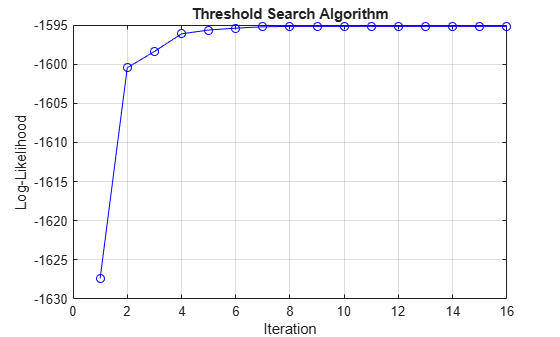
The plot indicates faster convergence, but at a reduced loglikelihood.

Compare the DGP and estimated threshold transitions.

varnames = ["DGP" "Unconstrained" "Constrained"];
array2table([MdlDGP.Switch.Levels, EstMdlSESTAR.Switch.Levels, EstMdlCon.Switch.Levels; ...
    MdlDGP.Switch.Rates, EstMdlSESTAR.Switch.Rates, EstMdlCon.Switch.Rates], ...
    VariableNames=varnames,RowNames=["MidLevel" "Rate"])

ans=2×3 table
                DGP    Unconstrained    Constrained
                ___    _____________    ___________

    MidLevel    2.5       2.6484          2.7977   
    Rate          5       4.6065          1.4487   

The estimation results are mixed. For example, the threshold parameter search appears to be inhibited by the equality constraints, resulting in less accurate estimates.

Compare the DGP and estimated AR parameters.

ARSubmodel1 = table(MdlDGP.Submodels(1).AR{1},EstMdlSESTAR.Submodels(1).AR{1}, ...
    EstMdlCon.Submodels(1).AR{1},VariableNames=varnames)

ARSubmodel1=2×3 table
       DGP           Unconstrained             Constrained     
    __________    ____________________    _____________________

    0.5      0     0.45497    0.071037     0.47106    -0.012461
      0    0.5    0.048204     0.49026    0.066586      0.51035

ARSubmodel2 = table([MdlDGP.Submodels(2).AR{1}; MdlDGP.Submodels(2).AR{2}], ...
    [EstMdlSESTAR.Submodels(2).AR{1}; EstMdlSESTAR.Submodels(2).AR{2}], ...
    [EstMdlCon.Submodels(2).AR{1}; EstMdlCon.Submodels(2).AR{2}], ...
    VariableNames=varnames)

ARSubmodel2=4×3 table
       DGP           Unconstrained            Constrained     
    __________    ____________________    ____________________

    0.3      0     0.33272    -0.14097     0.18716    -0.10112
      0    0.3    -0.15145     0.29089    -0.12179     0.25292
    0.4      0     0.35391     0.40149     0.33386     0.45529
      0    0.4     0.51186     0.36939     0.56162     0.37272

The AR parameter estimates show a mix of both improved and reduced accuracy under the equality constraints.

Summarize the estimation results.

summarize(EstMdlCon)

Description
2-Dimensional tsVAR Model with 2 Submodels

Switch
Transition Type: normal
Estimated Levels: 2.798
Estimated Rates: 1.449

Fit
Effective Sample Size: 498 
Number of Estimated Parameters: 12 
Number of Constrained Parameters: 10 
LogLikelihood: -1595.169 
AIC: 3214.338 
BIC: 3264.865 

Submodels
                           Estimate     StandardError    TStatistic      PValue  
                           _________    _____________    __________    __________

    State 1 Constant(1)            1             0             Inf              0
    State 1 Constant(2)           -1             0            -Inf              0
    State 1 AR{1}(1,1)       0.47106      0.075253          6.2597     3.8577e-10
    State 1 AR{1}(2,1)      0.066586      0.072189         0.92239        0.35633
    State 1 AR{1}(1,2)     -0.012461      0.042098        -0.29599        0.76724
    State 1 AR{1}(2,2)       0.51035      0.040384          12.638     1.3115e-36
    State 1 Beta(1,1)            0.3             0             Inf              0
    State 1 Beta(2,1)           -0.3             0            -Inf              0
    State 2 Constant(1)            2             0             Inf              0
    State 2 Constant(2)           -2             0            -Inf              0
    State 2 AR{1}(1,1)       0.18716      0.057629          3.2476      0.0011638
    State 2 AR{1}(2,1)      -0.12179      0.055283          -2.203       0.027594
    State 2 AR{1}(1,2)      -0.10112       0.05479         -1.8455        0.06496
    State 2 AR{1}(2,2)       0.25292       0.05256          4.8121     1.4932e-06
    State 2 AR{2}(1,1)       0.33386      0.060951          5.4776     4.3122e-08
    State 2 AR{2}(2,1)       0.56162      0.058469          9.6054     7.5852e-22
    State 2 AR{2}(1,2)       0.45529      0.057332          7.9413      2.001e-15
    State 2 AR{2}(2,2)       0.37272      0.054997          6.7771     1.2259e-11
    State 2 Beta(1,1)            0.5             0             Inf              0
    State 2 Beta(2,1)           -0.5             0            -Inf              0
    State 2 Beta(1,2)            0.2             0             Inf              0
    State 2 Beta(2,2)           -0.2             0            -Inf              0

Likelihood surfaces for the mixture densities of switching models, such as the negative sum-of-squares function evaluated by estimate, can have steep ridges and flat basins with highly contrasting directional derivatives, leading search algorithms to local maxima [2] [3]. In general, estimate is sensitive to the following characteristics:

• How well the model describes the data

• How well the data samples the submodels

• How large the sample size is

• How many parameters are estimated

• How the search is initiated and constrained

In practice, you can control only some of these parameters, and heuristic adjustments that lead to improved estimates are case-dependent.

Supporting Functions

This function displays all SESTAR model DGP values and estimates.

function compareEstimates(MdlDGP,EstMdl)
    fprintf("\nThreshold parameters:\n")
    disp([MdlDGP.Switch.Levels EstMdl.Switch.Levels; ...
        MdlDGP.Switch.Rates EstMdl.Switch.Rates])
    
    fprintf("\n\nSubmodel constants:\n")
    disp([MdlDGP.Submodels(1).Constant EstMdl.Submodels(1).Constant; ...
        MdlDGP.Submodels(2).Constant EstMdl.Submodels(2).Constant])
    
    fprintf("\n\nSubmodel(1) AR coefficients:\n")
    disp([MdlDGP.Submodels(1).AR{:} EstMdl.Submodels(1).AR{:}])
    
    fprintf("\n\nSubmodel(2) AR coefficients:\n")
    disp([MdlDGP.Submodels(2).AR{1} EstMdl.Submodels(2).AR{1}; ...
        MdlDGP.Submodels(2).AR{2} EstMdl.Submodels(2).AR{2}])
    
    fprintf("\n\nSubmodel(1) regression coefficients:\n")
    disp([MdlDGP.Submodels(1).Beta EstMdl.Submodels(1).Beta])
    
    fprintf("\n\nSubmodel(2) regression coefficients:\n")
    disp([MdlDGP.Submodels(2).Beta EstMdl.Submodels(2).Beta])
    
    fprintf("\n\nInnovations covariances:\n")
    disp([MdlDGP.Submodels(1).Covariance EstMdl.Submodels(1).Covariance; ...
        MdlDGP.Submodels(2).Covariance EstMdl.Submodels(2).Covariance])
end

References

[1] Chan, Kung-Sik, and Howell Tong. “On Estimating Thresholds in Autoregressive Models.” Journal of Time Series Analysis 7 (May 1986): 179–90. https://doi.org/10.1111/j.1467-9892.1986.tb00501.x.

[2] Hamilton, James D. Time Series Analysis. Princeton, NJ: Princeton University Press, 1994.

[3] van Dijk, Dick. Smooth Transition Models: Extensions and Outlier Robust Inference. Rotterdam, Netherlands: Tinbergen Institute Research Series, 1999.