Forecast a Conditional Variance Model
This example shows how to forecast a conditional variance model using forecast.
Load the data and specify the model.
Load the Deutschmark/British pound foreign exchange rate data included with the toolbox, and convert to returns. For numerical stability, convert returns to percentage returns.
load Data_MarkPound
r  = price2ret(Data);
pR = 100*r;
T  = length(r);
Specify and fit a GARCH(1,1) model.
Mdl = garch(1,1);
EstMdl = estimate(Mdl,pR);
    GARCH(1,1) Conditional Variance Model (Gaussian Distribution):

                 Value      StandardError    TStatistic      PValue
                ________    _____________    __________    __________

    Constant    0.010868      0.0012972        8.3779      5.3898e-17
    GARCH{1}     0.80452       0.016038        50.162               0
    ARCH{1}      0.15432       0.013852        11.141      7.9447e-29
Generate MMSE forecasts.
Use the fitted model to generate MMSE forecasts over a 200-period horizon. Use the observed return series as presample data. By default, forecast infers the corresponding presample conditional variances. Compare the asymptote of the variance forecast to the theoretical unconditional variance of the GARCH(1,1) model.
v = forecast(EstMdl,200,pR);
sig2 = EstMdl.Constant/(1-EstMdl.GARCH{1}-EstMdl.ARCH{1});

figure
plot(v,'r','LineWidth',2)
hold on
plot(ones(200,1)*sig2,'k--','LineWidth',1.5)
xlim([0,200])
title('Forecast Conditional Variance')
legend('Forecast','Theoretical','Location','SouthEast')
hold off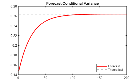
The MMSE forecasts converge to the theoretical unconditional variance after about 160 steps.