forecast
Forecast conditional variances from conditional variance models
Syntax
Description
V = forecast(Mdl,numperiods,Y0)V of the fully
specified, univariate conditional variance model Mdl, over
a numperiods forecast horizon. The model
Mdl can be a garch, egarch, or gjr model object. The forecasts
represent the continuation of the conditional variances associated with the
presample data in the numeric array Y0.
Tbl2 = forecast(Mdl,numperiods,Tbl1)Tbl2 containing the paths of
MMSE conditional variance variable forecasts of the model
Mdl over a numperiods forecast
horizon. forecast uses the table or timetable of
presample data Tbl1 to initialize the response
series. (since R2023a)
To initialize the forecast, forecast selects the
response variable named in Mdl.SeriesName or the sole
variable in Tbl1. To select a different response variable
in Tbl1 to initialize the forecasts, use the
PresampleResponseVariable name-value argument.
[___] = forecast(___,
specifies options using one or more name-value arguments in
addition to any of the input argument combinations in previous syntaxes.
Name,Value)forecast returns the output argument combination for the
corresponding input arguments. For example, forecast(Mdl,10,Y0,V0=v0)
initializes the conditional variances for the forecast using the presample data
in v0.
Examples
Forecast the conditional variance of simulated data over a 30-period horizon. Supply a vector of presample response data.
Simulate 100 observations from a GARCH(1,1) model with known parameters.
Mdl = garch(Constant=0.02,GARCH=0.8,ARCH=0.1);
rng("default") % For reproducibility
[v,y] = simulate(Mdl,100);
Forecast the conditional variances over a 30-period horizon. Specify the simulated response data. Plot the forecasts.
vF = forecast(Mdl,30,y);

figure
plot(v,"-b")
hold on
plot(101:130,vF,"r--",LineWidth=2);
title("Forecasted Conditional Variances")
legend("Simulated presample","Forecasts")
hold off
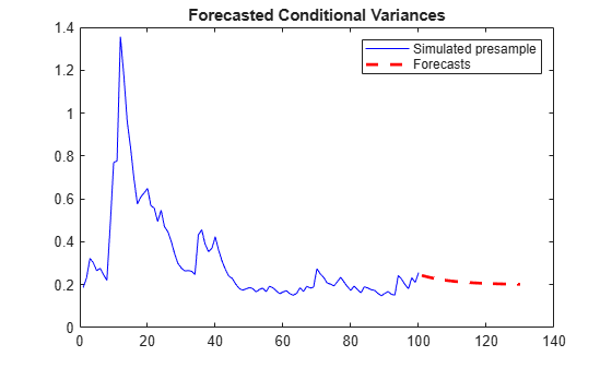
Forecasts converge asymptotically to the unconditional innovation variance.
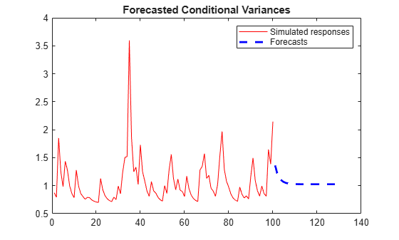
Forecast the conditional variance of simulated data over a 30-period horizon.
Simulate 100 observations from an EGARCH(1,1) model with known parameters.
Mdl = egarch(Constant=0.01,GARCH=0.6,ARCH=0.2, ...
    Leverage=-0.2);
rng("default") % For reproducibility
[v,y] = simulate(Mdl,100);
Forecast the conditional variance over a 30-period horizon. Specify the simulated data as presample responses. Plot the forecasts.
VF1 = forecast(Mdl,30,y);

figure
plot(v,"r-")
hold on
plot(101:130,VF1,"b--",LineWidth=2);
title("Forecasted Conditional Variances")
legend("Simulated responses","Forecasts")
hold off
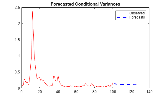
Forecast the conditional variance of simulated data over a 30-period horizon.
Simulate 100 observations from a GJR(1,1) model with known parameters.
Mdl = gjr(Constant=0.01,GARCH=0.6,ARCH=0.2, ...
    Leverage=0.2);
rng("default") % For reproducibility
[v,y] = simulate(Mdl,100);
Forecast the conditional variances over a 30-period horizon. Specify the simulated presample responses. Plot the forecasts.
vF = forecast(Mdl,30,y);

figure
plot(v,"r")
hold on
plot(101:130,vF,'b--',LineWidth=2);
title("Forecasted Conditional Variances")
legend("Observed","Forecasts")
hold off
Since R2023a
Forecast the conditional variance of the average weekly closing NASDAQ returns from fitted GARCH(1,1), EGARCH(1,1) and GJR(1,1) models.
Load the U.S. equity indices data Data_EquityIdx.mat.
load Data_EquityIdxThe timetable DataTimeTable contains the daily NASDAQ closing prices, among other indices.
Compute the weekly average closing prices of all timetable variables.
DTTW = convert2weekly(DataTimeTable,Aggregation="mean");Compute the weekly percent returns and their sample mean.
DTTRet = price2ret(DTTW);
DTTRet.Interval = [];
DTTRet.NASDAQ = DTTRet.NASDAQ*100;
T = height(DTTRet)
T =
626
meanRet = mean(DTTRet.NASDAQ)
meanRet =
0.0330
figure
plot(DTTRet.Time,100*DTTRet.NASDAQ);
hold on
yline(100*meanRet,'--r')
title("Daily NASDAQ Returns");
xlabel("Date");
ylabel("Return (%)");
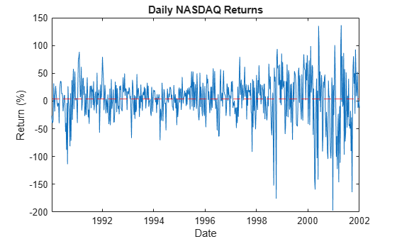
The variance of the series seems to change. This change is an indication of volatility clustering. The conditional mean model offset is very close to zero.
When you plan to supply a timetable, you must ensure it has all the following characteristics:
The selected response variable is numeric and does not contain any missing values.
The timestamps in the
Timevariable are regular, and they are ascending or descending.
Remove all missing values from the timetable, relative to the NASDAQ returns series.
DTTRet = rmmissing(DTTRet,DataVariables="NASDAQ");
numobs = height(DTTRet)
numobs = 626
Because all sample times have observed NASDAQ returns, rmmissing does not remove any observations.
Determine whether the sampling timestamps have a regular frequency and are sorted.
areTimestampsRegular = isregular(DTTRet,"weeks")areTimestampsRegular = logical
1
areTimestampsSorted = issorted(DTTRet.Time)
areTimestampsSorted = logical
   1
areTimestampsRegular = 1 indicates that the timestamps of DTTRet represent a regular weekly sample. areTimestampsSorted = 1 indicates that the timestamps are sorted.
Fit GARCH(1,1), EGARCH(1,1), and GJR(1,1) models to the data. By default, the software sets the conditional mean model offset to zero.
MdlGARCH = garch(1,1);
MdlEGARCH = egarch(1,1);
MdlGJR = gjr(1,1);

EstMdlGARCH = estimate(MdlGARCH,DTTRet,ResponseVariable="NASDAQ");
    GARCH(1,1) Conditional Variance Model (Gaussian Distribution):

                  Value      StandardError    TStatistic      PValue
                _________    _____________    __________    ___________

    Constant    0.0030629      0.0011827        2.5897        0.0096065
    GARCH{1}      0.86501        0.02911        29.715      4.8912e-194
    ARCH{1}       0.11835       0.024582        4.8144       1.4765e-06
EstMdlEGARCH = estimate(MdlEGARCH,DTTRet,ResponseVariable="NASDAQ");
    EGARCH(1,1) Conditional Variance Model (Gaussian Distribution):

                     Value      StandardError    TStatistic      PValue
                   _________    _____________    __________    __________

    Constant       -0.081262      0.030237        -2.6875       0.0071983
    GARCH{1}         0.95557       0.01335         71.579               0
    ARCH{1}           0.2768      0.052237          5.299      1.1645e-07
    Leverage{1}     -0.10519      0.025542        -4.1185      3.8142e-05
EstMdlGJR = estimate(MdlGJR,DTTRet,ResponseVariable="NASDAQ");
    GJR(1,1) Conditional Variance Model (Gaussian Distribution):

                     Value      StandardError    TStatistic      PValue
                   _________    _____________    __________    __________

    Constant       0.0069063      0.0020036         3.447       0.0005668
    GARCH{1}         0.78545       0.043862        17.907      1.0334e-71
    ARCH{1}         0.090637       0.034313        2.6415       0.0082543
    Leverage{1}      0.18663       0.054402        3.4305       0.0006025
Forecast the conditional variance for 20 weeks using the fitted models. Use the observed returns as presample innovations for the forecasts.
fh = 20;
DTTVFGARCH = forecast(EstMdlGARCH,fh,DTTRet, ...
    PresampleResponseVariable="NASDAQ");
DTTVFEGARCH = forecast(EstMdlEGARCH,fh,DTTRet, ...
    PresampleResponseVariable="NASDAQ");
DTTVFGJR= forecast(EstMdlGJR,fh,DTTRet, ...
    PresampleResponseVariable="NASDAQ");
The forecasted conditional variance variables are called Y_Variance in each returned timetable.
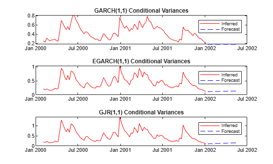
Plot the forecasts along with the conditional variances inferred from the data.
DTTVGARCH = infer(EstMdlGARCH,DTTRet,ResponseVariable="NASDAQ");
DTTVEGARCH = infer(EstMdlEGARCH,DTTRet,ResponseVariable="NASDAQ");
DTTVGJR = infer(EstMdlGJR,DTTRet,ResponseVariable="NASDAQ");

figure
tiledlayout(3,1)
nexttile
plot(DTTRet.Time(end-100:end),DTTVGARCH.Y_Variance(end-100:end), ...
    "r",DTTVFGARCH.Time,DTTVFGARCH.Y_Variance,"b--")
legend("Inferred","Forecast",Location="northeast")
title("GARCH(1,1) Conditional Variances")
nexttile
plot(DTTRet.Time(end-100:end),DTTVEGARCH.Y_Variance(end-100:end),"r", ...
    DTTVFEGARCH.Time,DTTVFEGARCH.Y_Variance,"b--")
legend("Inferred","Forecast",Location="northeast")
title("EGARCH(1,1) Conditional Variances")
nexttile
plot(DTTRet.Time(end-100:end),DTTVGJR.Y_Variance(end-100:end),"r", ...
    DTTVFGJR.Time,DTTVFGJR.Y_Variance,'b--')
legend("Inferred","Forecast",Location="northeast")
title("GJR(1,1) Conditional Variances")
Plot conditional variance forecasts for the next 500 weeks after the sample.
fh = 500;
DTTVF1000GARCH = forecast(EstMdlGARCH,fh,DTTRet, ...
    PresampleResponseVariable="NASDAQ");
DTTVF1000EGARCH = forecast(EstMdlEGARCH,fh,DTTRet, ...
    PresampleResponseVariable="NASDAQ");
DTTVF1000GJR= forecast(EstMdlGJR,fh,DTTRet, ...
    PresampleResponseVariable="NASDAQ");
figure
plot(DTTVF1000GARCH.Time,DTTVF1000GARCH.Y_Variance,'b',...
    DTTVF1000EGARCH.Time,DTTVF1000EGARCH.Y_Variance,'r',...
    DTTVF1000GJR.Time,DTTVF1000GJR.Y_Variance,'k')
legend("GARCH Forecast","EGARCH Foecast","GJR Forecast",Location="northeast")
title("Long-Run Conditional Variance Forecast")
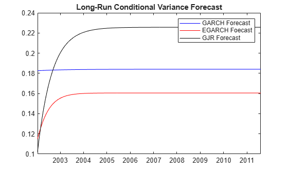
The forecasts converge asymptotically to the unconditional variances of their respective processes.
Input Arguments
Name-Value Arguments
Output Arguments
More About
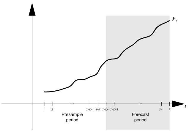
Time base partitions for forecasting are
two disjoint, contiguous intervals of the time base; each interval contains time
series data for forecasting a dynamic model. The forecast
period (forecast horizon) is a numperiods
length partition at the end of the time base during which
forecast generates forecasts V from
the dynamic model Mdl. The presample
period is the entire partition occurring before the forecast period.
forecast can require observed responses (or innovations)
Y0 or conditional variances V0 in the
presample period to initialize the dynamic model for forecasting. The model
structure determines the types and amounts of required presample
observations.
A common practice is to fit a dynamic model to a portion of the data set, then
validate the predictability of the model by comparing its forecasts to observed
responses. During forecasting, the presample period contains the data to which the
model is fit, and the forecast period contains the holdout sample for validation.
Suppose that yt is an observed response
series. Consider forecasting conditional variances from a dynamic model of
yt
numperiods = K periods. Suppose that the
dynamic model is fit to the data in the interval [1,T –
K] (for more details, see estimate). This figure shows the time base partitions for
forecasting.
For example, to generate forecasts Y from a GARCH(0,2) model,
forecast requires presample responses (innovations)
Y0 = to initialize the model. The 1-period-ahead forecast requires both
observations, whereas the 2-periods-ahead forecast requires
yT –
K and the 1-period-ahead forecast
V(1). forecast generates all other
forecasts by substituting previous forecasts for lagged responses in the
model.
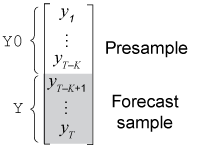
Dynamic models containing a GARCH component can require presample conditional
variances. Given enough presample responses, forecast infers
the required presample conditional variances. This figure shows the arrays of
required observations for this case, with corresponding input and output
arguments.
Algorithms
If the conditional variance model
Mdlhas an offset (Mdl.Offset),forecastsubtracts it from the specified presample responses to obtain presample innovations. Subsequently,forecastuses to initialize the conditional variance model for forecasting.forecastsets the number of sample paths to forecastnumpathsto the maximum number of columns among the specified presample response and conditional variance data sets. All presample data sets must have eithernumpaths> 1 columns or one column. Otherwise,forecastissues an error. For example, ifY0has five columns, representing five paths, thenV0can either have five columns or one column. IfV0has one column, thenforecastappliesV0to each path.
References
[1] Bollerslev, T. “Generalized Autoregressive Conditional Heteroskedasticity.” Journal of Econometrics. Vol. 31, 1986, pp. 307–327.
[2] Bollerslev, T. “A Conditionally Heteroskedastic Time Series Model for Speculative Prices and Rates of Return.” The Review of Economics and Statistics. Vol. 69, 1987, pp. 542–547.
[3] Box, G. E. P., G. M. Jenkins, and G. C. Reinsel. Time Series Analysis: Forecasting and Control. 3rd ed. Englewood Cliffs, NJ: Prentice Hall, 1994.
[4] Enders, W. Applied Econometric Time Series. Hoboken, NJ: John Wiley & Sons, 1995.
[5] Engle, R. F. “Autoregressive Conditional Heteroskedasticity with Estimates of the Variance of United Kingdom Inflation.” Econometrica. Vol. 50, 1982, pp. 987–1007.
[6] Glosten, L. R., R. Jagannathan, and D. E. Runkle. “On the Relation between the Expected Value and the Volatility of the Nominal Excess Return on Stocks.” The Journal of Finance. Vol. 48, No. 5, 1993, pp. 1779–1801.
[7] Hamilton, J. D. Time Series Analysis. Princeton, NJ: Princeton University Press, 1994.
[8] Nelson, D. B. “Conditional Heteroskedasticity in Asset Returns: A New Approach.” Econometrica. Vol. 59, 1991, pp. 347–370.