gctest

Block-wise Granger causality and block exogeneity tests

Syntax

h = gctest(Y1,Y2)

h = gctest(Y1,Y2,Y3)

h = gctest(___,Name,Value)

[h,pvalue,stat,cvalue] = gctest(___)

Description

The gctest function conducts a block-wise Granger causality test by accepting sets of time series data representing the "cause" and "effect" multivariate response variables in the test. gctest supports the inclusion of optional endogenous conditioning variables in the model for the test.

To conduct the leave-one-out, exclude-all, and block-wise Granger causality tests on the response variables of a fully specified VAR model (represented by a varm model object), see gctest.

h = gctest(Y1,Y2) returns the test decision h from conducting a block-wise Granger causality test for assessing whether a set of time series variables Y1 Granger-causes a distinct set of the time series variables Y2. The gctest function conducts tests in the vector autoregression (VAR) framework and treats Y1 and Y2 as response (endogenous) variables during testing.

h = gctest(Y1,Y2,Y3) conducts a 1-step Granger causality test for Y1 and Y2, conditioned on a distinct set of time series variables Y3. The variable Y3 is endogenous in the underlying VAR model, but gctest does not consider it a "cause" or an "effect" in the test.

h = gctest(___,Name,Value) specifies options using one or more name-value arguments in addition to the input argument combinations in previous syntaxes. For example, Test="f",NumLags=2 specifies conducting an F test that compares the residual sum of squares between restricted and unrestricted VAR(2) models for all response variables.

[h,pvalue,stat,cvalue] = gctest(___) additionally returns the p-value pvalue, test statistic stat, and critical value cvalue for the test.

Examples

Conduct Granger Causality Test

Conduct a Granger causality test to assess whether the M1 money supply has an impact on the predictive distribution of the consumer price index (CPI).

Load the US macroeconomic data set Data_USEconModel.mat.

load Data_USEconModel

The data set includes the MATLAB® timetable DataTimeTable, which contains 14 variables measured from Q1 1947 through Q1 2009. M1SL is the table variable containing the M1 money supply, and CPIAUCSL is the table variable containing the CPI. For more details, enter Description at the command line.

Visually assess whether the series are stationary by plotting them in the same figure.

figure;
yyaxis left
plot(DataTimeTable.Time,DataTimeTable.CPIAUCSL)
ylabel("CPI");
yyaxis right
plot(DataTimeTable.Time,DataTimeTable.M1SL);
ylabel("Money Supply");

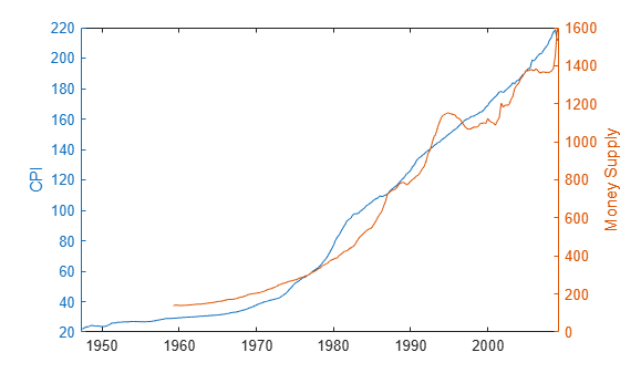
Both series are nonstationary.

Stabilize the series by converting them to rates.

m1slrate = price2ret(DataTimeTable.M1SL);
inflation = price2ret(DataTimeTable.CPIAUCSL);

Assume that a VAR(1) model is an appropriate multivariate model for the rates. Conduct a default Granger causality test to assess whether the M1 money supply rate Granger-causes the inflation rate.

h = gctest(m1slrate,inflation)

h = logical
   1

The test decision h is 1, which indicates the rejection of the null hypothesis that the M1 money supply rate does not Granger-cause inflation.

Test Series for Feedback

Time series undergo feedback when they Granger-cause each other. Assess whether the US inflation and M1 money supply rates undergo feedback.

Load the US macroeconomic data set Data_USEconModel.mat. Convert the price series to returns.

load Data_USEconModel
inflation = price2ret(DataTimeTable.CPIAUCSL);
m1slrate = price2ret(DataTimeTable.M1SL);

Conduct a Granger causality test to assess whether the inflation rate Granger-causes the M1 money supply rate. Assume that an underlying VAR(1) model is appropriate for the two series. The default level of significance $\alpha$ for the test is 0.05. Because this example conducts two tests, decrease $\alpha$ by half for each test to achieve a family-wise level of significance of 0.05.

hIRgcM1 = gctest(inflation,m1slrate,Alpha=0.025)

hIRgcM1 = logical
   1

The test decision hIRgcM1 = 1 indicates rejection of the null hypothesis of noncausality. There is enough evidence to suggest that the inflation rate Granger-causes the M1 money supply rate at 0.025 level of significance.

Conduct another Granger causality test to assess whether the M1 money supply rate Granger-causes the inflation rate.

hM1gcIR = gctest(m1slrate,inflation,Alpha=0.025)

hM1gcIR = logical
   0

The test decision hM1gcIR = 0 indicates that the null hypothesis of noncausality should not be rejected. There is not enough evidence to suggest that the M1 money supply rate Granger-causes the inflation rate at 0.025 level of significance.

Because not enough evidence exists to suggest that the inflation rate Granger-causes the M1 money supply rate, the two series do not undergo feedback.

Conduct 1-Step Granger Causality Test Conditioned on Variable

Assess whether the US gross domestic product (GDP) Granger-causes CPI conditioned on the M1 money supply.

Load the US macroeconomic data set Data_USEconModel.mat.

load Data_USEconModel

The variables GDP and GDPDEF of DataTimeTable are the US GDP and its deflator with respect to year 2000 dollars, respectively. Both series are nonstationary.

Convert the M1 money supply and CPI to rates. Convert the US GDP to the real GDP rate.

m1slrate = price2ret(DataTimeTable.M1SL);
inflation = price2ret(DataTimeTable.CPIAUCSL);
rgdprate = price2ret(DataTimeTable.GDP./DataTimeTable.GDPDEF);

Assume that a VAR(1) model is an appropriate multivariate model for the rates. Conduct a Granger causality test to assess whether the real GDP rate has an impact on the predictive distribution of the inflation rate, conditioned on the M1 money supply. The inclusion of a conditional variable forces gctest to conduct a 1-step Granger causality test.

h = gctest(rgdprate,inflation,m1slrate)

h = logical
   0

The test decision h is 0, which indicates failure to reject the null hypothesis that the real GDP rate is not a 1-step Granger-cause of inflation when you account for the M1 money supply rate.

gctest includes the M1 money supply rate as a response variable in the underlying VAR(1) model, but it does not include the M1 money supply in the computation of the test statistics.

Conduct the test again, but without conditioning on the M1 money supply rate.

h = gctest(rgdprate,inflation)

h = logical
   0

The test result is the same as before, suggesting that the real GDP rate does not Granger-cause inflation at all periods in a forecast horizon and regardless of whether you account for the M1 money supply rate in the underlying VAR(1) model.

Adjust Number of Lags for Underlying VAR Model

By default, gctest assumes an underlying VAR(1) model for all specified response variables. However, a VAR(1) model might be an inappropriate representation of the data. For example, the model might not capture all the serial correlation present in the variables.

To specify a more complex underlying VAR model, you can increase the number of lags by specifying the NumLags name-value argument of gctest.

Consider the Granger causality tests conducted in Conduct 1-Step Granger Causality Test Conditioned on Variable. Load the US macroeconomic data set Data_USEconModel.mat. Convert the M1 money supply and CPI to rates. Convert the US GDP to the real GDP rate.

load Data_USEconModel
m1slrate = price2ret(DataTimeTable.M1SL);
inflation = price2ret(DataTimeTable.CPIAUCSL);
rgdprate = price2ret(DataTimeTable.GDP./DataTimeTable.GDPDEF);

Preprocess the data by removing all missing observations (indicated by NaN).

idx = sum(isnan([m1slrate inflation rgdprate]),2) < 1;
m1slrate = m1slrate(idx);
inflation = inflation(idx);
rgdprate = rgdprate(idx);
T = numel(m1slrate); % Total sample size

Fit VAR models, with lags ranging from 1 to 4, to the real GDP and inflation rate series. Initialize each fit by specifying the first four observations. Store the Akaike information criteria (AIC) of the fits.

numseries = 2;
numlags = (1:4)';
nummdls = numel(numlags);

% Partition time base.
maxp = max(numlags); % Maximum number of required presample responses
idxpre = 1:maxp;
idxest = (maxp + 1):T;

% Preallocation
EstMdl(1:nummdls) = varm(numseries,0);
aic = zeros(nummdls,1);

% Fit VAR models to data.
Y0 = [rgdprate(idxpre) inflation(idxpre)]; % Presample
Y = [rgdprate(idxest) inflation(idxest)];  % Estimation sample
for j = 1:numel(numlags)
    Mdl = varm(numseries,numlags(j));
    Mdl.SeriesNames = ["rGDP" "Inflation"];
    EstMdl(j) = estimate(Mdl,Y,Y0=Y0);
    results = summarize(EstMdl(j));
    aic(j) = results.AIC;
end

p = numlags(aic == min(aic))

p = 3

A VAR(3) model yields the best fit.

Assess whether the real GDP rate Granger-causes inflation. gctest removes $\mathit{p}$ observations from the beginning of the input data to initialize the underlying VAR($\mathit{p}$) model for estimation. Prepend only the required $\mathit{p}$ = 3 presample observations to the estimation sample. Specify the concatenated series as input data. Return the $\mathit{p}$-value of the test.

rgdprate3 = [Y0((end - p + 1):end,1); Y(:,1)];
inflation3 = [Y0((end - p + 1):end,2); Y(:,2)];
[h,pvalue] = gctest(rgdprate3,inflation3,NumLags=p)

h = logical
   1

pvalue = 7.7741e-04

The $\mathit{p}$-value is approximately 0.0008, indicating the existence of strong evidence to reject the null hypothesis of noncausality, that is, that the three real GDP rate lags in the inflation rate equation are jointly zero. Given the VAR(3) model, there is enough evidence to suggest that the real GDP rate Granger-causes at least one future value of the inflation rate.

Alternatively, you can conduct the same test by passing the estimated VAR(3) model (represented by the varm model object in EstMdl(3)), to the object function gctest. Specify a block-wise test and the "cause" and "effect" series names.

h = gctest(EstMdl(3),Type="block-wise", ...
    Cause="rGDP",Effect="Inflation")

                         H0                          Decision      Distribution    Statistic      PValue      CriticalValue
    ____________________________________________    ___________    ____________    _________    __________    _____________

    "Exclude lagged rGDP in Inflation equations"    "Reject H0"     "Chi2(3)"       16.799      0.00077741       7.8147    

h = logical
   1

Address Integrated Series During Testing

If you are testing integrated series for Granger causality, then the Wald test statistic does not follow a ${\chi }^2$ or $\mathit{F}$ distribution, and test results can be unreliable. However, you can implement the Granger causality test in [5] by specifying the maximum integration order among all the variables in the system using the Integration name-value argument.

Consider the Granger causality tests conducted in Conduct 1-Step Granger Causality Test Conditioned on Variable. Load the US macroeconomic data set Data_USEconModel.mat and take the log of real GDP and CPI.

load Data_USEconModel
cpi = log(DataTimeTable.CPIAUCSL);
rgdp = log(DataTimeTable.GDP./DataTimeTable.GDPDEF);

Assess whether the real GDP Granger-causes CPI. Assume the series are $\mathit{I}\left(1\right)$, or order-1 integrated. Also, specify an underlying VAR(3) model and the $\mathit{F}$ test. Return the test statistic and $\mathit{p}$-value.

[h,pvalue,stat] = gctest(rgdp,cpi,NumLags=3, ...
    Integration=1,Test="f")

h = logical
   1

pvalue = 0.0031

stat = 4.7557

The $\mathit{p}$-value = 0.0031, indicating the existence of strong evidence to reject the null hypothesis of noncausality, that is, that the three real GDP lags in the CPI equation are jointly zero. Given the VAR(3) model, there is enough evidence to suggest that real GDP Granger-causes at least one future value of the CPI.

In this case, the test augments the VAR(3) model with an additional lag. In other words, the model is a VAR(4) model. However, gctest tests only whether the first three lags are 0.

Test for Block Exogeneity

Time series are block exogenous if they do not Granger-cause any other variables in a multivariate system. Test whether the effective federal funds rate is block exogenous with respect to the real GDP, personal consumption expenditures, and inflation rates.

Load the US macroeconomic data set Data_USEconModel.mat. Convert the price series to returns.

load Data_USEconModel
inflation = price2ret(DataTimeTable.CPIAUCSL);
rgdprate = price2ret(DataTimeTable.GDP./DataTimeTable.GDPDEF);
pcerate = price2ret(DataTimeTable.PCEC);

Test whether the federal funds rate is nonstationary by conducting an augmented Dickey-Fuller test. Specify that the alternative model has a drift term and an $\mathit{F}$ test.

StatTbl = adftest(DataTimeTable,DataVariable="FEDFUNDS",Model="ard")

StatTbl=1×8 table
                h       pValue      stat      cValue     Lags    Alpha     Model      Test 
              _____    ________    _______    _______    ____    _____    _______    ______

    Test 1    false    0.071419    -2.7257    -2.8751     0      0.05     {'ARD'}    {'T1'}

The test decision h = 0 indicates that the null hypothesis that the series has a unit root should not be rejected, at 0.05 significance level.

To stabilize the federal funds rate series, apply the first difference to it.

dfedfunds = diff(DataTimeTable.FEDFUNDS);

Assume a 4-D VAR(3) model for the four series. Assess whether the federal funds rate is block exogenous with respect to the real GDP, personal consumption expenditures, and inflation rates. Conduct an $\mathit{F}$-based Wald test, and return the $\mathit{p}$-value, test statistic, and critical value.

cause = dfedfunds;
effects = [inflation rgdprate pcerate];
[hgc,pvalue,stat,cvalue] = gctest(cause,effects,NumLags=2,Test="f")

hgc = logical
   1

pvalue = 4.1619e-10

stat = 10.4383

cvalue = 2.1426

The test decision hgc = 1 indicates that the null hypothesis that the federal funds rate is block exogenous should be rejected. This result suggests that the federal funds rate Granger-causes at least one of the other variables in the system.

To determine which variables the federal funds rate Granger-causes, you can run a leave-one-out test. For more details, see gctest.

Input Arguments

Y1 — Data for response variables representing Granger-causes

numeric vector | numeric matrix

Data for the response variables representing the Granger-causes in the test, specified as a numobs1-by-1 numeric vector or a numobs1-by-numseries1 numeric matrix. numobs1 is the number of observations and numseries1 is the number of time series variables.

Row t contains the observation in time t, the last row contains the latest observation. Y1 must have enough rows to initialize and estimate the underlying VAR model. gctest uses the first NumLags observations to initialize the model for estimation.

Columns correspond to distinct time series variables.

Data Types: double | single

Y2 — Data for response variables affected by Granger-causes

numeric vector | numeric matrix

Data for response variables affected by the Granger-causes in the test, specified as a numobs2-by-1 numeric vector or a numobs2-by-numseries2 numeric matrix. numobs2 is the number of observations in the data and numseries2 is the number of time series variables.

Row t contains the observation in time t, the last row contains the latest observation. Y2 must have enough rows to initialize and estimate the underlying VAR model. gctest uses the first NumLags observations to initialize the model for estimation.

Columns correspond to distinct time series variables.

Data Types: double | single

Y3 — Data for conditioning response variables

numeric vector | numeric matrix

Data for conditioning response variables, specified as a numobs3-by-1 numeric vector or a numobs3-by-numseries3 numeric matrix. numobs3 is the number of observations in the data and numseries3 is the number of time series variables.

Row t contains the observation in time t, the last row contains the latest observation. Y3 must have enough rows to initialize and estimate the underlying VAR model. gctest uses the first NumLags observations to initialize the model for estimation.

Columns correspond to distinct time series variables.

If you specify Y3, then Y1, Y2, and Y3 represent the response variables in the underlying VAR model. gctest assesses whether Y1 is a 1-step Granger-cause of Y2.

Data Types: double | single

Name-Value Arguments

Specify optional pairs of arguments as Name1=Value1,...,NameN=ValueN, where Name is the argument name and Value is the corresponding value. Name-value arguments must appear after other arguments, but the order of the pairs does not matter.

Before R2021a, use commas to separate each name and value, and enclose Name in quotes.

Example: Alpha=0.10,NumLags=2 specifies a 0.10 significance level for the test and uses an underlying VAR(2) model for all response variables.

NumLags — Number of lagged responses

1 (default) | nonnegative integer

Number of lagged responses to include in the underlying VAR model for all response variables, specified as a nonnegative integer. The resulting underlying model is a VAR(NumLags) model.

Example: NumLags=2

Data Types: double | single

Integration — Maximum order of integration

0 (default) | nonnegative integer

Maximum order of integration among all response variables, specified as a nonnegative integer.

To address integration, gctest augments the VAR(NumLags) model by adding additional lagged responses beyond NumLags to all equations during estimation. For more details, see [5] and [3].

Example: Integration=1

Data Types: double | single

Constant — Flag indicating inclusion of model intercepts

true (default) | false

Flag indicating the inclusion of model intercepts (constants) in the underlying VAR model, specified as a value in this table.

Value	Description
true	All equations in the underlying VAR model have an intercept. gctest estimates the intercepts with all other estimable parameters.
false	All underlying VAR model equations do not have an intercept. gctest sets all intercepts to 0.

Example: Constant=false

Data Types: logical

Trend — Flag indicating inclusion of linear time trends

false (default) | true

Flag indicating the inclusion of linear time trends in the underlying VAR model, specified as a value in this table.

Value	Description
true	All equations in the underlying VAR model have a linear time trend. gctest estimates the linear time trend coefficients with all other estimable parameters.
false	All underlying VAR model equations do not have a linear time trend.

Example: Trend=false

Data Types: logical

X — Predictor data

numeric matrix

Predictor data for the regression component in the underlying VAR model, specified as a numeric matrix containing numpreds columns. numpreds is the number of predictor variables.

Row t contains the observation in time t, and the last row contains the latest observation. gctest does not use the regression component in the presample period. X must have at least as many observations as the number of observations used by gctest after the presample period. Specifically, X must have at least numobs – Mdl.P observations, where numobs = min([numobs1 numobs2 numobs3]). If you supply more rows than necessary, gctest uses the latest observations only.

Columns correspond to individual predictor variables. gctest treats predictors as exogenous. All predictor variables are present in the regression component of each response equation.

By default, gctest excludes a regression component from all equations.

Data Types: double | single

Alpha — Significance level

0.05 (default) | numeric scalar in (0,1)

Significance level for the test, specified as a numeric scalar in (0,1).

Example: Alpha=0.1

Data Types: double | single

Test — Test statistic distribution under the null hypothesis

"chi-square" (default) | "f"

Test statistic distribution under the null hypothesis, specified as a value in this table.

Value	Description
"chi-square"	gctest derives outputs from conducting a χ2 test.
"f"	gctest derives outputs from conducting an F test.

For test statistic forms, see [4].

Example: Test="f"

Data Types: char | string

Output Arguments

h — Block-wise Granger causality test decision

logical scalar

Block-wise Granger causality test decision, returned as a logical scalar.

• h = 1 indicates rejection of H₀.

  • If you specify the conditioning response data Y3, then sufficient evidence exists to suggest that the response variables represented in Y1 are 1-step Granger-causes of the response variables represented in Y2, conditioned on the response variables represented in Y3.

  • Otherwise, sufficient evidence exists to suggest that the variables in Y1 are h-step Granger-causes of the variables in Y2 for some h ≥ 0. In other words, Y1 is block endogenous with respect to Y2.

• h = 0 indicates failure to reject H₀.

  • If you specify Y3, then the variables in Y1 are not 1-step Granger-causes of the variables in Y2, conditioned on Y3.

  • Otherwise, Y1 does not Granger-cause Y2. In other words, there is not enough evidence to reject block exogeneity of Y1 with respect to Y2.

pvalue — p-value

numeric scalar

p-value, returned as a numeric scalar.

stat — Test statistic

numeric scalar

Test statistic, returned as a numeric scalar.

cvalue — Critical value

numeric scalar

Critical value for the significance level Alpha, returned as a numeric scalar.

More About

Granger Causality Test

The Granger causality test is a statistical hypothesis test that assesses whether past and present values of a set of m₁ = numseries1 time series variables y_1,t, called the "cause" variables, affect the predictive distribution of a distinct set of m₂ = numseries2 time series variables y_2,t, called the "effect" variables. The impact is a reduction in forecast mean squared error (MSE) of y_2,t. If past values of y_1,t affect y_{2,t + h}, then y_1,t is an h-step Granger-cause of y_2,t. In other words, y_1,t Granger-causes y_2,t if y_1,t is an h-step Granger-cause of y_2,t for all h ≥ 1.

Consider a stationary VAR(p) model for [y_1,t y_2,t]:

$$\left[\begin{array}{c}{y}_{1,t}\\ y_{2,t}\end{array}\right]=c+\delta t+\beta x_t+\left[\begin{array}{cc}{\Phi }_{11,1}& {\Phi }_{12,1}\\ {\Phi }_{21,1}& {\Phi }_{22,1}\end{array}\right]\left[\begin{array}{c}{y}_{1,t-1}\\ y_{2,t-1}\end{array}\right]+\mathrm{...}+\left[\begin{array}{cc}{\Phi }_{11,p}& {\Phi }_{12,p}\\ {\Phi }_{21,p}& {\Phi }_{22,p}\end{array}\right]\left[\begin{array}{c}{y}_{1,t-p}\\ y_{2,t-p}\end{array}\right]+\left[\begin{array}{c}{\epsilon }_{1,t}\\ {\epsilon }_{2,t}\end{array}\right].$$

Assume the following conditions:

• Future values cannot inform past values.

• y_1,t uniquely informs y_2,t (no other variable has the information to inform y_2,t).

If Φ_21,1 = … = Φ_21,p = 0_m1,m2, then y_1,t is not the block-wise Granger cause of y_{2,t + h}, for all h ≥ 1 and where 0_m2,m1 is an m₂-by-m₁ matrix of zeros. Also, y_1,t is block exogenous with respect to y_2,t. Consequently, the block-wise Granger causality test hypotheses are:

$$\begin{array}{l}{H}_0:{\Phi }_{21,1}=\mathrm{...}={\Phi }_{21,p}=0_{m_2,m_1}\\ H_1:\exists j\in \{1,\mathrm{...},p\}\ni {\Phi }_{21,j}\ne 0_{m_2,m_1}.\end{array}$$

H₁ implies that at least one h ≥ 1 exists such that y_1,t is an h-step Granger-cause of y_2,t.

gctest conducts χ²-based or F-based Wald tests (see 'Test'). For test statistic forms, see [4].

Distinct conditioning endogenous variables y_3,t can be included in the system (see Y3). In this case, the VAR(p) model is:

$$\left[\begin{array}{c}{y}_{1,t}\\ \begin{array}{l}{y}_{2,t}\\ y_{3,t}\end{array}\end{array}\right]=c+\delta t+\beta x_t+\left[\begin{array}{ccc}{\Phi }_{11,1}& {\Phi }_{12,1}& {\Phi }_{13,1}\\ {\Phi }_{21,1}& {\Phi }_{22,1}& {\Phi }_{23,1}\\ {\Phi }_{31,1}& {\Phi }_{32,1}& {\Phi }_{33,1}\end{array}\right]\left[\begin{array}{c}{y}_{1,t-1}\\ \begin{array}{l}{y}_{2,t-1}\\ y_{3,t-1}\end{array}\end{array}\right]+\mathrm{...}+\left[\begin{array}{ccc}{\Phi }_{11,p}& {\Phi }_{12,p}& {\Phi }_{13,p}\\ {\Phi }_{21,p}& {\Phi }_{22,p}& {\Phi }_{23,p}\\ {\Phi }_{31,p}& {\Phi }_{32,p}& {\Phi }_{33,p}\end{array}\right]\left[\begin{array}{c}{y}_{1,t-p}\\ \begin{array}{l}{y}_{2,t-p}\\ y_{3,t-p}\end{array}\end{array}\right]+\left[\begin{array}{c}{\epsilon }_{1,t}\\ \begin{array}{l}{\epsilon }_{2,t}\\ {\epsilon }_{3,t}\end{array}\end{array}\right].$$

gctest does not test the parameters associated with the conditioning variables. The test assesses only whether y_1,t is an 1-step Granger-cause of y_2,t.

Vector Autoregression Model

A vector autoregression (VAR) model is a stationary multivariate time series model consisting of a system of m equations of m distinct response variables as linear functions of lagged responses and other terms.

A VAR(p) model in difference-equation notation and in reduced form is

$$y_t=c+{\Phi }_1{y}_{t-1}+{\Phi }_2{y}_{t-2}+\mathrm{...}+{\Phi }_p{y}_{t-p}+\beta x_t+\delta t+{\epsilon }_t.$$

• y_t is a numseries-by-1 vector of values corresponding to numseries response variables at time t, where t = 1,...,T. The structural coefficient is the identity matrix.

• c is a numseries-by-1 vector of constants.

• Φ_j is a numseries-by-numseries matrix of autoregressive coefficients, where j = 1,...,p and Φ_p is not a matrix containing only zeros.

• x_t is a numpreds-by-1 vector of values corresponding to numpreds exogenous predictor variables.

• β is a numseries-by-numpreds matrix of regression coefficients.

• δ is a numseries-by-1 vector of linear time-trend values.

• ε_t is a numseries-by-1 vector of random Gaussian innovations, each with a mean of 0 and collectively a numseries-by-numseries covariance matrix Σ. For t ≠ s, ε_t and ε_s are independent.

Condensed and in lag operator notation, the system is

$$\Phi (L)y_t=c+\beta x_t+\delta t+{\epsilon }_t,$$

where $$\Phi (L)=I-{\Phi }_{1}L-{\Phi }_2{L}^2-\mathrm{...}-{\Phi }_p{L}^p$$, Φ(L)y_t is the multivariate autoregressive polynomial, and I is the numseries-by-numseries identity matrix.

For example, a VAR(1) model containing two response series and three exogenous predictor variables has this form:

$$\begin{array}{l}{y}_{1,t}=c_1+{\varphi }_{11}{y}_{1,t-1}+{\varphi }_{12}{y}_{2,t-1}+{\beta }_{11}{x}_{1,t}+{\beta }_{12}{x}_{2,t}+{\beta }_{13}{x}_{3,t}+{\delta }_{1}t+{\epsilon }_{1,t}\\ y_{2,t}=c_2+{\varphi }_{21}{y}_{1,t-1}+{\varphi }_{22}{y}_{2,t-1}+{\beta }_{21}{x}_{1,t}+{\beta }_{22}{x}_{2,t}+{\beta }_{23}{x}_{3,t}+{\delta }_{2}t+{\epsilon }_{2,t}.\end{array}$$

References

[1] Granger, C. W. J. "Investigating Causal Relations by Econometric Models and Cross-Spectral Methods." Econometrica. Vol. 37, 1969, pp. 424–459.

[2] Hamilton, James D. Time Series Analysis. Princeton, NJ: Princeton University Press, 1994.

[3] Dolado, J. J., and H. Lütkepohl. "Making Wald Tests Work for Cointegrated VAR Systems." Econometric Reviews. Vol. 15, 1996, pp. 369–386.

[4] Lütkepohl, Helmut. New Introduction to Multiple Time Series Analysis. New York, NY: Springer-Verlag, 2007.

[5] Toda, H. Y., and T. Yamamoto. "Statistical Inferences in Vector Autoregressions with Possibly Integrated Processes." Journal of Econometrics. Vol. 66, 1995, pp. 225–250.

Version History

Introduced in R2019a