Main Content

lmtest

Lagrange multiplier test of model specification

Description

example

h = lmtest(score,ParamCov,dof) returns a logical value with the rejection decision from conducting a Lagrange multiplier test of model specification at the 5% significance level. lmtest constructs the test statistic using the input evaluated score function, estimated parameter covariance, and degrees of freedom.

example

h = lmtest(score,ParamCov,dof,alpha) returns the rejection decision of the Lagrange multiplier test conducted at an input significance level.

  • If the input evaluated score function and estimated parameter covariance are length k cell arrays, all other arguments must be length k vectors or scalars. lmtest treats each cell as a separate test, and returns a vector of rejection decisions.

  • If the input evaluated score function is a row cell array, lmtest returns a row vector.

example

[h,pValue] = lmtest(___) returns the p-value for the hypothesis test, using any of the input arguments in the previous syntaxes.

example

[h,pValue,stat,cValue] = lmtest(___) returns the test statistic and critical value for the hypothesis test.

Examples

collapse all

Compare AR model specifications for a simulated response series using lmtest.

Consider the AR(3) model:

yt=1+0.9yt-1-0.5yt-2+0.4yt-3+εt,

where εt is Gaussian with mean 0 and variance 1. Specify this model using arima.

Mdl = arima('Constant',1,'Variance',1,'AR',{0.9,-0.5,0.4});

Mdl is a fully specified, AR(3) model.

Simulate presample and effective sample responses from Mdl.

T = 100;
rng(1);               % For reproducibility
n = max(Mdl.P,Mdl.Q); % Number of presample observations
y = simulate(Mdl,T + n);

y is a a random path from Mdl that includes presample observations.

Specify the restricted model:

yt=c+ϕ1yt-1+ϕ2yt-2+εt,

where εt is Gaussian with mean 0 and variance σ2.

Mdl0 = arima(3,0,0);
Mdl0.AR{3} = 0;

The structure of Mdl0 is the same as Mdl. However, every parameter is unknown, except that ϕ3=0. This is an equality constraint during estimation.

Estimate the restricted model using the simulated data (y).

[EstMdl0,EstParamCov] = estimate(Mdl0,y((n+1):end),...
    'Y0',y(1:n),'display','off');
phi10 = EstMdl0.AR{1};
phi20 = EstMdl0.AR{2};
phi30 = 0;
c0 = EstMdl0.Constant;
phi0 = [c0;phi10;phi20;phi30];
v0 = EstMdl0.Variance;

EstMdl0 contains the parameter estimates of the restricted model.

lmtest requires the unrestricted model score evaluated at the restricted model estimates. The unrestricted model gradient is

l(ϕ1,ϕ2,ϕ3,c,σ2;yt,...,yt-3)c=1σ2(yt-c-ϕ1yt-1-ϕ2yt-2-ϕ3yt-3)

l(ϕ1,ϕ2,ϕ3,c,σ2;yt,...,yt-3)ϕj=1σ2(yt-c-ϕ1yt-1-ϕ2yt-2-ϕ3yt-3)yt-j

l(ϕ1,ϕ2,ϕ3,c,σ2;yt,...,yt-3)σ2=-12σ2+12σ4(yt-c-ϕ1yt-1-ϕ2yt-2-ϕ3yt-3)2.

MatY = lagmatrix(y,1:3);
LagY = MatY(all(~isnan(MatY),2),:);
cGrad = (y((n+1):end)-[ones(T,1),LagY]*phi0)/v0;
phi1Grad = ((y((n+1):end)-[ones(T,1),LagY]*phi0).*LagY(:,1))/v0;
phi2Grad = ((y((n+1):end)-[ones(T,1),LagY]*phi0).*LagY(:,2))/v0;
phi3Grad = ((y((n+1):end)-[ones(T,1),LagY]*phi0).*LagY(:,3))/v0;
vGrad = -1/(2*v0)+((y((n+1):end)-[ones(T,1),LagY]*phi0).^2)/(2*v0^2);
Grad = [cGrad,phi1Grad,phi2Grad,phi3Grad,vGrad]; % Gradient matrix

score = sum(Grad)'; % Score under the restricted model

Evaluate the unrestricted parameter covariance estimator using the restricted MLEs and the outer product of gradients (OPG) method.

EstParamCov0 = inv(Grad'*Grad);
dof = 1; % Number of model restrictions

Test the null hypothesis that ϕ3=0 at a 1% significance level using lmtest.

[h,pValue] = lmtest(score,EstParamCov0,dof,0.1)
h = logical
   1

pValue = 2.2524e-09

pValue is close to 0, which suggests that there is strong evidence to reject the restricted, AR(2) model in favor of the unrestricted, AR(3) model.

Compare two model specifications for simulated education and income data. The unrestricted model has the following loglikelihood:

l(β,ρ)=-nlogΓ(ρ)+ρk=1nlogβk+(ρ-1)k=1nlog(yk)-k=1nykβk,

where

  • βk=1β+xk.

  • xk is the number of grades that person k completed.

  • yk is the income (in thousands of USD) of person k.

That is, the income of person k given the number of grades that person k completed is Gamma distributed with shape ρ and rate βi. The restricted model sets ρ=1, which implies that the income of person k given the number of grades person k completed is exponentially distributed with mean β+xi.

The restricted model is H0:ρ=1. In order to compare this model to the unrestricted model, you require:

  • The gradient vector of the unrestricted model

  • The maximum likelihood estimate (MLE) under the restricted model

  • The parameter covariance estimator evaluated under the MLEs of the restricted model

Load the data.

load Data_Income1
x = DataTable.EDU;
y = DataTable.INC;

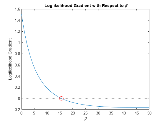
Estimate the restricted model parameters by maximizing l(ρ,β) with respect to β subject to the restriction ρ=1. The gradient of l(ρ,β) is

l(ρ,β)β=i=1T(yiβi2-ρβi)

l(ρ,β)ρ=-TΨ(ρ)+i=1T(logβiyi),

where Ψ(ρ) is the digamma function.

rho0 = 1; % Restricted rho
dof = 1;  % Number of restrictions
dLBeta = @(beta) sum(y./((beta + x).^2) - rho0./(beta + x));...
    % Anonymous gradient function

[betaHat0,fVal,exitFlag] = fzero(dLBeta,0)
betaHat0 = 15.6027
fVal = 2.7756e-17
exitFlag = 1
beta = [0:0.1:50];
plot(beta,arrayfun(dLBeta,beta))
hold on
plot([beta(1);beta(end)],zeros(2,1),'k:')
plot(betaHat0,fVal,'ro','MarkerSize',10)
xlabel('{\beta}')
ylabel('Loglikelihood Gradient')
title('{\bf Loglikelihood Gradient with Respect to \beta}')
hold off

The gradient with respect to β (dLBeta) is decreasing, which suggests that there is a local maximum at its root. Therefore, betaHat0 is the MLE for the restricted model. fVal indicates that the value of the gradient is very close to 0 at betaHat0. The exit flag (exitFlag) is 1, which indicates that fzero found a root of the gradient without a problem.

Estimate the parameter covariance under the restricted model using the outer product of gradients (OPG).

rGradient = [-rho0./(betaHat0+x)+y.*(betaHat0+x).^(-2),...
      log(y./(betaHat0+x))-psi(rho0)];    % Gradient per unit
rScore = sum(rGradient)';                 % Score function
rEstParamCov = inv(rGradient'*rGradient); % Parameter covariance estimate

Test the unrestricted model against the restricted model using the Lagrange multiplier test.

[h,pValue] = lmtest(rScore,rEstParamCov,dof)
h = logical
   1

pValue = 7.4744e-05

pValue is close to 0, which indicates that there is strong evidence to suggest that the unrestricted model fits the data better than the restricted model.

Test whether there are significant ARCH effects in a simulated response series using lmtest. The parameter values in this example are arbitrary.

Specify the AR(1) model with an ARCH(1) variance:

yt=0.9yt-1+εt,

where

  • εt=wtht.

  • ht=1+0.5εt-12.

  • wt is Gaussian with mean 0 and variance 1.

VarMdl = garch('ARCH',0.5,'Constant',1);
Mdl = arima('Constant',0,'Variance',VarMdl,'AR',0.9);

Mdl is a fully specified, AR(1) model with an ARCH(1) variance.

Simulate presample and effective sample responses from Mdl.

T = 100;
rng(1);  % For reproducibility
n = 2;   % Number of presample observations required for the gradient
[y,ep,v] = simulate(Mdl,T + n);

ep is the random path of innovations from VarMdl. The software filters ep through Mdl to yield the random response path y.

Specify the restricted model and assume that the AR model constant is 0:

yt=c+ϕ1yt-1+εt,

where ht=α0+α1εt-12.

VarMdl0 = garch(0,1);
VarMdl0.ARCH{1} = 0;
Mdl0 = arima('ARLags',1,'Constant',0,'Variance',VarMdl0);

The structure of Mdl0 is the same as Mdl. However, every parameter is unknown, except for the restriction α1=0. These are equality constraints during estimation. You can interpret Mdl0 as an AR(1) model with the Gaussian innovations that have mean 0 and constant variance.

Estimate the restricted model using the simulated data (y).

psI = 1:n;             % Presample indices
esI = (n + 1):(T + n); % Estimation sample indices

[EstMdl0,EstParamCov] = estimate(Mdl0,y(esI),...
    'Y0',y(psI),'E0',ep(psI),'V0',v(psI),'display','off');
phi10 = EstMdl0.AR{1};
alpha00 = EstMdl0.Variance.Constant;

EstMdl0 contains the parameter estimates of the restricted model.

lmtest requires the unrestricted model score evaluated at the restricted model estimates. The unrestricted model loglikelihood function is

l(ϕ1,α0,α1)=t=2T(-0.5log(2π)-0.5loght-εt22ht),

where εt=yt-ϕ1yt-1. The unrestricted gradient is

l(ϕ1,α0,α1)α=t=2T12htztft,

where zt=[1,εt-12] and ft=εt2ht-1. The information matrix is

I=12ht2t=2Tztzt.

Under the null, restricted model, ht=h0=αˆ0 for all t, where αˆ0 is the estimate from the restricted model analysis.

Evaluate the gradient and information matrix under the restricted model. Estimate the parameter covariance by inverting the information matrix.

e = y - phi10*lagmatrix(y,1);
eLag1Sq = lagmatrix(e,1).^2;
h0 = alpha00;
ft = (e(esI).^2/h0 - 1);
zt = [ones(T,1),eLag1Sq(esI)]';

score0 = 1/(2*h0)*zt*ft;        % Score function
InfoMat0 = (1/(2*h0^2))*(zt*zt');
EstParamCov0 = inv(InfoMat0);   % Estimated parameter covariance
dof = 1;                        % Number of model restrictions

Test the null hypothesis that α1=0 at the 5% significance level using lmtest.

[h,pValue] = lmtest(score0,EstParamCov0,dof)
h = logical
   1

pValue = 4.0443e-06

pValue is close to 0, which suggests that there is evidence to reject the restricted AR(1) model in favor of the unrestricted AR(1) model with an ARCH(1) variance.

Input Arguments

collapse all

Unrestricted model loglikelihood gradients evaluated at the restricted model parameter estimates, specified as a vector or cell vector.

  • For a single test, score can be a p-vector or a singleton cell array containing a p-by-1 vector. p is the number of parameters in the unrestricted model.

  • For conducting k > 1 tests, score must be a length k cell array. Cell j must contain one pj-by-1 vector that corresponds to one independent test. pj is the number of parameters in the unrestricted model of test j.

Data Types: double | cell

Parameter covariance estimate, specified as a symmetric matrix of cell array of symmetric matrices. ParamCov is the unrestricted model parameter covariance estimator evaluated at the restricted model parameter estimates.

  • For a single test, ParamCov can be a p-by-p matrix or singleton cell array containing a p-by-p matrix. p is the number of parameters in the unrestricted model.

  • For conducting k > 1 tests, ParamCov must be a length k cell array. Cell j must contain one pj-by-pj matrix that corresponds to one independent test. pj is the number of parameters in the unrestricted model of test j.

Data Types: double | cell

Degrees of freedom for the asymptotic, chi-square distribution of the test statistics, specified as a positive integer or vector of positive integers.

For each corresponding test, the elements of dof:

  • Are the number of model restrictions

  • Should be less than the number of parameters in the unrestricted model

When conducting k > 1 tests,

  • If dof is a scalar, then the software expands it to a k-by-1 vector.

  • If dof is a vector, then it must have length k.

Nominal significance levels for the hypothesis tests, specified as a scalar or vector.

Each element of alpha must be greater than 0 and less than 1.

When conducting k > 1 tests,

  • If alpha is a scalar, then the software expands it to a k-by-1 vector.

  • If alpha is a vector, then it must have length k.

Data Types: double

Output Arguments

collapse all

Test rejection decisions, returned as a logical value or vector of logical values with a length equal to the number of tests that the software conducts.

  • h = 1 indicates rejection of the null, restricted model in favor of the alternative, unrestricted model.

  • h = 0 indicates failure to reject the null, restricted model.

Test statistic p-values, returned as a scalar or vector with a length equal to the number of tests that the software conducts.

Test statistics, returned as a scalar or vector with a length equal to the number of tests that the software conducts.

Critical values determined by alpha, returned as a scalar or vector with a length equal to the number of tests that the software conducts.

More About

collapse all

Lagrange Multiplier Test

This test compares specifications of nested models by assessing the significance of restrictions to an extended model with unrestricted parameters. The test statistic (LM) is

LM=SVS,

where

  • S is the gradient of the unrestricted loglikelihood function, evaluated at the restricted parameter estimates (score), i.e.,

    S=l(θ)θ|θ=θ^0,MLE.

  • V is the covariance estimator for the unrestricted model parameters, evaluated at the restricted parameter estimates.

If LM exceeds a critical value in its asymptotic distribution, then the test rejects the null, restricted (nested) model in favor of the alternative, unrestricted model.

The asymptotic distribution of LM is chi-square. Its degrees of freedom (dof) is the number of restrictions in the corresponding model comparison. The nominal significance level of the test (alpha) determines the critical value (cValue).

Tips

  • lmtest requires the unrestricted model score and parameter covariance estimator evaluated at parameter estimates for the restricted model. For example, to compare competing, nested arima models:

    1. Analytically compute the score and parameter covariance estimator based on the innovation distribution.

    2. Use estimate to estimate the restricted model parameters.

    3. Evaluate the score and covariance estimator at the restricted model estimates.

    4. Pass the evaluated score, restricted covariance estimate, and the number of restrictions (i.e., the degrees of freedom) into lmtest.

  • If you find estimating parameters in the unrestricted model difficult, then use lmtest. By comparison:

    • waldtest only requires unrestricted parameter estimates.

    • lratiotest requires both unrestricted and restricted parameter estimates.

Algorithms

  • lmtest performs multiple, independent tests when inputs are cell arrays.

    • If the gradients and covariance estimates are the same for all tests, but the restricted parameter estimates vary, then lmtest “tests down” against multiple restricted models.

    • If the gradients and covariance estimates vary, but the restricted parameter estimates do not, then lmtest “tests up” against multiple unrestricted models.

    • Otherwise, lmtest compares model specifications pair-wise.

  • alpha is nominal in that it specifies a rejection probability in the asymptotic distribution. The actual rejection probability can differ from the nominal significance. Lagrange multiplier tests tend to under-reject for small values of alpha, and over-reject for large values of alpha.

    Lagrange multiplier tests typically yield lower rejection errors than likelihood ratio and Wald tests.

References

[1] Davidson, R. and J. G. MacKinnon. Econometric Theory and Methods. Oxford, UK: Oxford University Press, 2004.

[2] Godfrey, L. G. Misspecification Tests in Econometrics. Cambridge, UK: Cambridge University Press, 1997.

[3] Greene, W. H. Econometric Analysis. 6th ed. Upper Saddle River, NJ: Pearson Prentice Hall, 2008.

[4] Hamilton, J. D. Time Series Analysis. Princeton, NJ: Princeton University Press, 1994.

Version History

Introduced in R2009a