smooth

Smoothed inference of operative latent states in Markov-switching dynamic regression data

Syntax

SS = smooth(Mdl,Y)

SS = smooth(Mdl,Y,Name,Value)

[SS,logL] = smooth(___)

Description

SS = smooth(Mdl,Y) returns smoothed state probabilities SS of the operative latent states in the regime-switching data Y. The Markov-switching dynamic regression model Mdl models the data. smooth performs a forward recursion using filter, and then performs the reverse recursion of Kim [5].

SS = smooth(Mdl,Y,Name,Value) uses additional options specified by one or more name-value arguments. For example, 'Y0',Y0 initializes the dynamic component of each submodel by using the presample response data Y0.

[SS,logL] = smooth(___) also returns the estimated loglikelihood logL using any of the input argument combinations in the previous syntaxes.

Examples

Compute Smoothed State Probabilities

Compute smoothed state probabilities from a two-state Markov-switching dynamic regression model for a 1-D response process. This example uses arbitrary parameter values for the data-generating process (DGP).

Create Fully Specified Model for DGP

Create a two-state discrete-time Markov chain model for the switching mechanism.

P = [0.9 0.1; 0.2 0.8];
mc = dtmc(P);

mc is a fully specified dtmc object.

For each state, create an AR(0) (constant only) model for the response process. Store the models in a vector.

mdl1 = arima('Constant',2,'Variance',3);
mdl2 = arima('Constant',-2,'Variance',1);
mdl = [mdl1; mdl2];

mdl1 and mdl2 are fully specified arima objects.

Create a Markov-switching dynamic regression model from the switching mechanism mc and the vector of submodels mdl.

Mdl = msVAR(mc,mdl);

Mdl is a fully specified msVAR object.

Simulate Data from DGP

smooth requires responses to compute smoothed state probabilities. Generate one random response and state path, both of length 30, from the DGP.

rng(1000); % For reproducibility
[y,~,sp] = simulate(Mdl,30);

Compute State Probabilities

Compute filtered and smoothed state probabilities from the Markov-switching model given the simulated response data.

fs = filter(Mdl,y);
ss = smooth(Mdl,y);

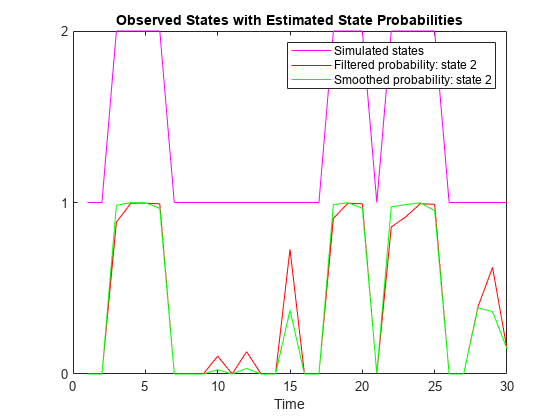
fs and ss are 30-by-2 matrices of filtered and smoothed state probabilities, respectively, for each period in the simulation horizon. Although the filtered state probabilities at time t (fs(t,:)) are based on the response data through time t (y(1:t)), the smoothed state probabilities at time t (ss(t,:)) are based on all observations.

Plot the simulated state path and the filtered and smoothed state probabilities on the same graph.

figure
plot(sp,'m')
hold on
plot(fs(:,2),'r')
plot(ss(:,2),'g')
yticks([0 1 2])
xlabel("Time")
title("Observed States with Estimated State Probabilities")
legend({'Simulated states','Filtered probability: state 2',...
    'Smoothed probability: state 2'})
hold off

Compute Smoothed Probabilities of Recession

Consider a two-state Markov-switching dynamic regression model of the postwar US real GDP growth rate. The model has the parameter estimates presented in [1].

Create Markov-Switching Dynamic Regression Model

Create a fully specified discrete-time Markov chain model that describes the regime switching mechanism. Label the regimes.

P = [0.92 0.08; 0.26 0.74];
mc = dtmc(P,'StateNames',["Expansion" "Recession"]);

Create separate, fully specified AR(0) models for the two regimes.

sigma = 3.34; % Homoscedastic models across states
mdl1 = arima('Constant',4.62,'Variance',sigma^2);
mdl2 = arima('Constant',-0.48,'Variance',sigma^2);
mdl = [mdl1 mdl2];

Create the Markov-switching dynamic regression model from the switching mechanism mc and the state-specific submodels mdl.

Mdl = msVAR(mc,mdl);

Mdl is a fully specified msVAR object.

Load and Preprocess Data

Load the US GDP data set. Convert serial dates to datetimes.

load Data_GDP
dt = datetime(dates,'ConvertFrom','datenum');

Data contains quarterly measurements of the US real GDP in the period 1947:Q1–2005:Q2. The period of interest in [1] is 1947:Q2–2004:Q2. For more details on the data set, enter Description at the command line.

Transform the data to an annualized rate series by:

1. Converting the data to a quarterly rate within the estimation period

2. Annualizing the quarterly rates

qrate = diff(Data(2:230))./Data(2:229); % Quarterly rate
arate = 100*((1 + qrate).^4 - 1);       % Annualized rate

The transformation drops the first observation.

Compute Smoothed State Probabilities

Compute smoothed state probabilities for the data and model. Display the smoothed state distribution for 1972:Q2.

SS = smooth(Mdl,arate);
SS(end,:)

ans = 1×2

    0.9396    0.0604

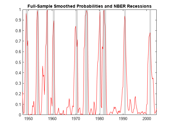
SS is a 228-by-2 matrix of smoothed state probabilities. Rows correspond to periods in the data arate, and columns correspond to the regimes.

Plot the smoothed probabilities of recession, as in [1], Figure 6.

figure
plot(dt(3:230),SS(:,2),'r')
recessionplot
title("Full-Sample Smoothed Probabilities and NBER Recessions")

Compute Smoothed State Probabilities from Model with VARX Submodels

Compute smoothed state probabilities from a three-state Markov-switching dynamic regression model for a 2-D VARX response process. This example uses arbitrary parameter values for the DGP.

Create Fully Specified Model for DGP

Create a three-state discrete-time Markov chain model for the switching mechanism.

P = [5 1 1; 1 5 1; 1 1 5];
mc = dtmc(P);

mc is a fully specified dtmc object. dtmc normalizes the rows of P so that they sum to 1.

For each state, create a fully specified VARX(0) model (constant and regression coefficient matrix only) for the response process. Specify different constant vectors across models. Specify the same regression coefficient for the two regressors, and specify the same covariance matrix. Store the VARX models in a vector.

% Constants
C1 = [1;-1];
C2 = [3;-3];
C3 = [5;-5];

% Regression coefficient
Beta = [0.2 0.1;0 -0.3];

% Covariance matrix
Sigma = [1.8 -0.4; -0.4 1.8];

% VARX submodels
mdl1 = varm('Constant',C1,'Beta',Beta,...
    'Covariance',Sigma);
mdl2 = varm('Constant',C2,'Beta',Beta,...
    'Covariance',Sigma);
mdl3 = varm('Constant',C3,'Beta',Beta,...
    'Covariance',Sigma);

mdl = [mdl1; mdl2; mdl3];

mdl contains three fully specified varm model objects.

For the DGP, create a fully specified Markov-switching dynamic regression model from the switching mechanism mc and the submodels mdl.

Mdl = msVAR(mc,mdl);

Mdl is a fully specified msVAR model.

Simulate Data from DGP

Simulate data for the two exogenous series by generating 30 observations from the standard 2-D Gaussian distribution.

rng(1) % For reproducibility
X = randn(30,2);

Generate one random response and state path, both of length 30, from the DGP. Specify the simulated exogenous data for the submodel regression components.

[Y,~,SP] = simulate(Mdl,30,'X',X);

Y is a 30-by-2 matrix of one simulated response path. SP is a 30-by-1 vector of one simulated state path.

Compute State Probabilities

Compute smoothed state probabilities from the DGP given the simulated response data.

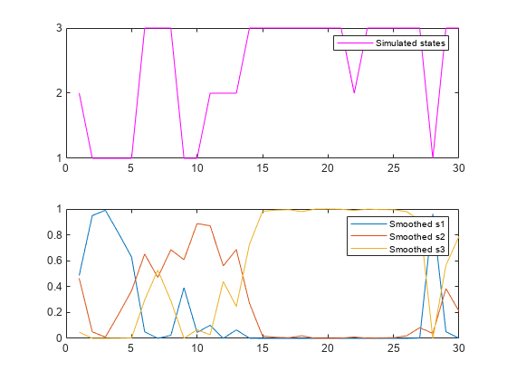
SS = smooth(Mdl,Y,'X',X);

SS is a 30-by-2 matrix of smoothed state probabilities for each period in the simulation horizon.

Plot the simulated state path and the smoothed state probabilities on subplots in the same figure.

figure
subplot(2,1,1)
plot(SP,'m')
yticks([1 2 3])
legend({'Simulated states'})
subplot(2,1,2)
plot(SS,'-')
legend({'Smoothed s1','Smoothed s2','Smoothed s3'})

Specify Presample Data

Consider the data in Compute Smoothed Probabilities of Recession, but assume that the period of interest is 1960:Q1–2004:Q2. Also, consider adding an autoregressive term to each submodel.

Create Partially Specified Model for Estimation

Create a partially specified Markov-switching dynamic regression model for estimation. Specify AR(1) submodels.

P = NaN(2);
mc = dtmc(P,'StateNames',["Expansion" "Recession"]);
mdl = arima(1,0,0);
Mdl = msVAR(mc,[mdl; mdl]);

Because the submodels are AR(1), each requires one presample observation to initialize its dynamic component for estimation.

Create Fully Specified Model Containing Initial Values

Create the model containing initial parameter values for the estimation procedure.

mc0 = dtmc(0.5*ones(2),'StateNames',["Expansion" "Recession"]);
submdl01 = arima('Constant',1,'Variance',1,'AR',0.001);
submdl02 = arima('Constant',-1,'Variance',1,'AR',0.001);
Mdl0 = msVAR(mc0,[submdl01; submdl02]);

Load and Preprocess Data

Load the data. Transform the entire set to an annualized rate series.

load Data_GDP
qrate = diff(Data)./Data(1:(end - 1)); 
arate = 100*((1 + qrate).^4 - 1);

Identify the presample and estimation sample periods using the dates associated with the annualized rate series. Because the transformation applies the first difference, you must drop the first observation date from the original sample.

dates = datetime(dates(2:end),'ConvertFrom','datenum',...
    'Format','yyyy:QQQ','Locale','en_US');
estPrd = datetime(["1960:Q2" "2004:Q2"],'InputFormat','yyyy:QQQ',...
    'Format','yyyy:QQQ','Locale','en_US');
idxEst = isbetween(dates,estPrd(1),estPrd(2));
idxPre = dates < estPrd(1); 

Estimate Model

Fit the model to the estimation sample data. Specify the presample observation.

arate0 = arate(idxPre);
arateEst = arate(idxEst);
EstMdl = estimate(Mdl,Mdl0,arateEst,'Y0',arate0);

EstMdl is a fully specified msVAR object.

Compute Smoothed State Probabilities

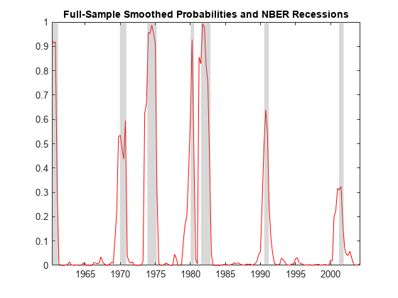
Compute smoothed state probabilities from the estimated model and data in the estimation period. Specify the presample observation. Plot the estimated probabilities of recession.

SS = smooth(EstMdl,arateEst,'Y0',arate0);

figure;
plot(dates(idxEst),SS(:,2),'r')
title("Full-Sample Smoothed Probabilities and NBER Recessions")
recessionplot

Return Loglikelihood for Data

Consider the model and data in Compute Smoothed Probabilities of Recession.

Create the fully specified Markov-switching model.

P = [0.92 0.08; 0.26 0.74];
mc = dtmc(P,'StateNames',["Expansion" "Recession"]);

sigma = 3.34;
mdl1 = arima('Constant',4.62,'Variance',sigma^2);
mdl2 = arima('Constant',-0.48,'Variance',sigma^2);
mdl = [mdl1; mdl2];

Mdl = msVAR(mc,mdl);

Load and preprocess the data.

load Data_GDP

qrate = diff(Data(2:230))./Data(2:229); 
arate = 100*((1 + qrate).^4 - 1);       

Compute smoothed state probabilities and the loglikelihood for the data and model.

[SS,logL] = smooth(Mdl,arate);
logL

logL = 
-640.3016

Input Arguments

Mdl — Fully specified Markov-switching dynamic regression model

msVAR model object

Fully specified Markov-switching dynamic regression model, specified as an msVAR model object returned by msVAR or estimate. Properties of a fully specified model object do not contain NaN values.

Y — Observed response data

numeric matrix

Observed response data, specified as a numObs-by-numSeries numeric matrix.

numObs is the sample size. numSeries is the number of response variables (Mdl.NumSeries).

Rows correspond to observations, and the last row contains the latest observation. Columns correspond to individual response variables.

Y represents the continuation of the presample response series in Y0.

Data Types: double

Name-Value Arguments

Specify optional pairs of arguments as Name1=Value1,...,NameN=ValueN, where Name is the argument name and Value is the corresponding value. Name-value arguments must appear after other arguments, but the order of the pairs does not matter.

Before R2021a, use commas to separate each name and value, and enclose Name in quotes.

Example: 'Y0',Y0,'X',X initializes the dynamic component of each submodel in Mdl by using the presample response data Y0, and includes a linear regression component in each submodel composed of the predictor data in X and the specified regression coefficients.

Y0 — Presample response data

numeric matrix

Presample response data, specified as the comma-separated pair consisting of 'Y0' and a numPreSampleObs-by-numSeries numeric matrix.

The number of presample observations numPreSampleObs must be sufficient to initialize the AR terms of all submodels. If numPreSampleObs exceeds the AR order of any state, smooth uses the latest observations. By default, Y0 is the initial segment of Y, which reduces the effective sample size.

Data Types: double

S0 — Initial state probabilities

nonnegative numeric vector

Initial state probabilities, specified as the comma-separated pair consisting of 'S0' and a nonnegative numeric vector of length numStates.

smooth normalizes S0 to produce a distribution.

By default, S0 is a steady-state distribution computed by asymptotics.

Example: 'S0',[0.2 0.2 0.6]

Example: 'S0',[0 1] specifies state 2 as the initial state.

Data Types: double

X — Predictor data

numeric matrix | cell vector of numeric matrices

Predictor data used to evaluate regression components in all submodels of Mdl, specified as the comma-separated pair consisting of 'X' and a numeric matrix or a cell vector of numeric matrices.

To use a subset of the same predictors in each state, specify X as a matrix with numPreds columns and at least numObs rows. Columns correspond to distinct predictor variables. Submodels use initial columns of the associated matrix, in order, up to the number of submodel predictors. The number of columns in the Beta property of Mdl.SubModels(j) determines the number of exogenous variables in the regression component of submodel j. If the number of rows exceeds numObs, then smooth uses the latest observations.

To use different predictors in each state, specify a cell vector of such matrices with length numStates.

By default, smooth ignores regression components in Mdl.

Data Types: double

Output Arguments

SS — Smoothed state probabilities

nonnegative numeric matrix

Smoothed state probabilities, returned as a numObs-by-numStates nonnegative numeric matrix.

logL — Estimated loglikelihood

numeric scalar

Estimated loglikelihood of the response data Y, returned as a numeric scalar.

Algorithms

smooth refines current estimates of the state distribution that filter produces by iterating backward from the full sample history Y.

References

[1] Chauvet, M., and J. D. Hamilton. "Dating Business Cycle Turning Points." In Nonlinear Analysis of Business Cycles (Contributions to Economic Analysis, Volume 276). (C. Milas, P. Rothman, and D. van Dijk, eds.). Amsterdam: Emerald Group Publishing Limited, 2006.

[2] Hamilton, J. D. "A New Approach to the Economic Analysis of Nonstationary Time Series and the Business Cycle." Econometrica. Vol. 57, 1989, pp. 357–384.

[3] Hamilton, J. D. "Analysis of Time Series Subject to Changes in Regime." Journal of Econometrics. Vol. 45, 1990, pp. 39–70.

[4] Hamilton, James D. Time Series Analysis. Princeton, NJ: Princeton University Press, 1994.

[5] Kim, C.-J. "Dynamic Linear Models with Markov Switching." Journal of Econometrics. Vol. 60, 1994, pp. 1–22.

Version History

Introduced in R2019b