Visualize Threshold Transitions
This example shows how to plot threshold transitions to compare transition function rates and view mixing rates of the threshold levels.
Compare Transition Function Rates
Consider defining discrete economic states based on the CPI-based Canadian inflation rate. Specifically:
Inflation is low when its rate is below 2%.
Inflation is moderate when its rate is at least 2% and below 8%.
Inflation is high when its rate is at least 8%.
Transitions are smooth and modeled using the logistic distribution.
The transition rate from low to moderate inflation is 3.5, and the rate from moderate to high inflation is 1.5.
Create threshold transitions representing the state space based on the CPI-based Canadian inflation rate. Assign names "Low", "Med", and "High" to the states.
ttL = threshold([2 8],Type="logistic",Rates=[3.5 1.5], ...
    StateNames=["Low" "Med" "High"]);
ttL is a threshold object that is a model for the state space of the inflation rate.
Compare transition rates at the levels by calling ttplot and specifying the "graph" plot type.
ttplot(ttL,Type="graph")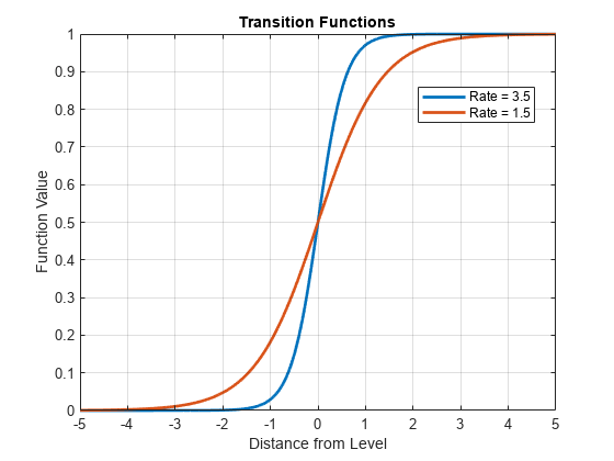
For comparison, ttplot centers the transition functions at level 0. In a threshold-switching model (tsVAR), a higher rate results in quicker mixing of submodel responses.
To plot the transition functions at their respective levels:
Evaluate the transition functions by passing the threshold transitions and a grid of transition variable data to
ttdata. By default,ttdataevaluates the transition functions at the corresponding levels.Plot the results with respect to the transition function data.
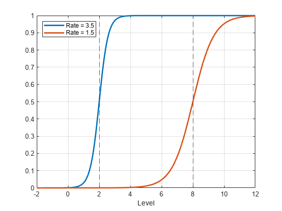
Plot the transition functions of ttL at their respective levels.
z = -2:0.01:12;    % Grid of transition variable data
n = numel(z);
f = ttdata(ttL,z);

plot(z,f,LineWidth=2)
xline(ttL.Levels,"--")
grid on
xlabel("Level")
legend(["Rate = 3.5" "Rate = 1.5"],Location="northwest")
View Mixing Levels
To view mixing levels at each transition, with the option of superimposing observed threshold variable data, use ttplot and specify the "gradient" plot type.
Plot the threshold transitions with the observed inflation rate series.
load Data_Canada
INF_C = DataTable.INF_C;    % Inflation rate (threshold variable)

figure
ttplot(ttL,Type="gradient",Data=INF_C)
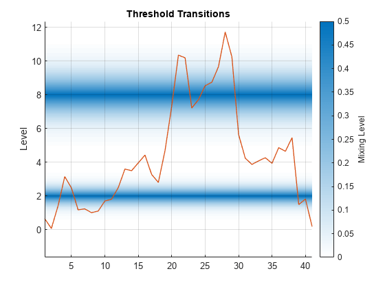
For transition function , the mixing level is the degree to which states on both sides of a level contribute to a response. The mixing level is .
Plot Exponential Transition Function
Discrete, normal, and logistic transition functions separate states at small and large values of a threshold variable . However, exponential transitions separate states at small and large values of , which gives the transitions a distinct shape and mixing characteristics.
Consider an arbitrary threshold variable. Create a threshold transition at level 1. Specify an exponential transition function with rate 1.5.
ttE = threshold(1,Type="exponential",Rates=1.5);Plot the transition function and mixing level of the threshold transition.
ttplot(ttE,Type="graph")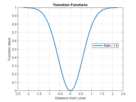
figure
ttplot(ttE,Type="gradient")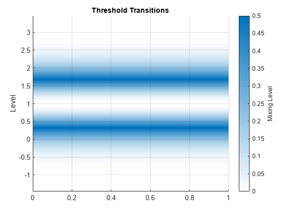
Exponential transitions can model deviations with inner and outer states, such as real exchange rates. According to the principle of purchasing power parity, large deviations from a parity level are expected to be eliminated more quickly than small ones. Because larger differences allow for larger profits, faster arbitrage results [1].