clearInstrumentationResults

Clear results logged by instrumented, compiled C code function

Syntax

clearInstrumentationResults('mex_fcn')

clearInstrumentationResults mex_fcn

clearInstrumentationResults all

Description

clearInstrumentationResults('mex_fcn') clears the results logged from calling the instrumented MEX function, mex_fcn.

clearInstrumentationResults mex_fcn is an alternative syntax for clearing the log.

clearInstrumentationResults all clears the results from all instrumented MEX functions.

Examples

Create Instrumented MEX Function

This example shows how to create an instrumented MEX function, run a test bench, then view logged results.

Define prototype input arguments.

n = 128;
x = complex(zeros(n,1));
w = fi_radix2twiddles(n);

Generate an instrumented MEX function. Use the -o option to specify the MEX function name. Use the -histogram option to compute histograms.

buildInstrumentedMex testfft -o testfft_instrumented -args {x,coder.Constant(w)} -histogram

If you have a MATLAB® Coder™ license, you can also add the -coder option. For example,

buildInstrumentedMex testfft -coder -o testfft_instrumented -args {x,w}

Like the fiaccel function, the buildInstrumentedMex function generates a MEX function. To generate C code, use the MATLAB® Coder™ codegen function.

Run a test file to record instrumentation results.

for i=1:20
   y = testfft_instrumented(randn(size(x)),w);
end

showInstrumentationResults testfft_instrumented

Use the showInstrumenationResults function to open the report. To view the simulation minimum and maximum values and whole number status, pause over a variable in the report. The variable information also displays in the Variables tab of the report.

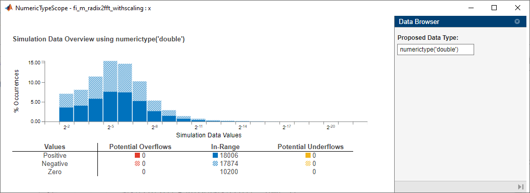
You can switch to the Data Type Visualizer tab to view a histogram of ranges for all the variables in the function. The histogram shows the data type ranges and logged ranges from simulation to help you quickly identify overflows. You can click on a histogram bin to see the associated variable information.

In this example, all of the logged values fall within their respective data type ranges. No overflows are detected.

Close the report, then use the clearInstrumentationResults function to clear the results log.

clearInstrumentationResults testfft_instrumented

Run a different test bench, then view the new instrumentation results.

for i=1:20
   y = testfft_instrumented(cast(rand(size(x))-0.5,'like',x),w);
end

showInstrumentationResults testfft_instrumented

To view the histogram for a variable, click the histogram icon in the Variables tab.

Close the histogram display, then use the clearInstrumentationResults function to clear the results log.

clearInstrumentationResults testfft_instrumented

Clear the MEX function.

clear testfft_instrumented

Input Arguments

mex_fcn — Instrumented MEX function

instrumented MEX function

Instrumented MEX function created using buildInstrumentedMex.

Version History

Introduced in R2011b