Air Traffic Control in Simulink
This example shows how to create a tracking system for an air traffic control center using a global nearest neighbor (GNN) tracker in Simulink. This example closely follows the Air Traffic Control MATLAB® example.
Overview of the Model
model = 'AirTrafficControlInSimulink';
open_system(model);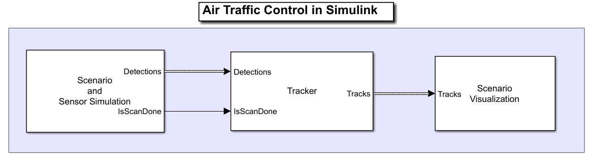
The model has three subsystems, each implementing a part of the workflow.
Scenario and Sensor Simulation
Tracker
Scenario Visualization
Scenario and Sensor Simulation
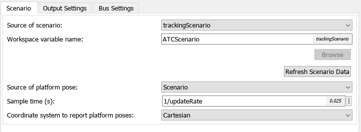
You create the scenario using the trackingScenario object. You add a platform to represent the ATC tower and add three platforms to represent three airliners. One airliner approaches the ATC from a long range, another departs, and the third is flying tangential to the tower. You add an airport surveillance radar (ASR) to the ATC tower platform. A typical ATC tower has a radar mounted 15 meters above the ground. This radar scans mechanically in azimuth at a fixed rate to provide 360-degree coverage in the vicinity of the ATC tower. You use the fusionRadarSensor object to model the radar. See the createATCScenario.m file in the example folder for more details on the configuration of the scenario and radar.
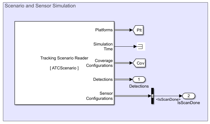
The Tracking Scenario Reader block reads the tracking scenario object from the MATLAB workspace and generates simulation data. You set the sample time for the block as the reciprocal of the update rate of the radar sensor. You configure the block to additionally output coverage configurations, detections, and sensor configurations from the scenario. You also specify an initial seed to have reproducible results.
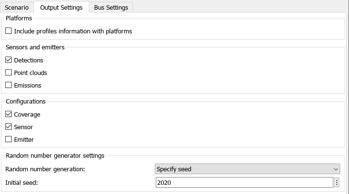
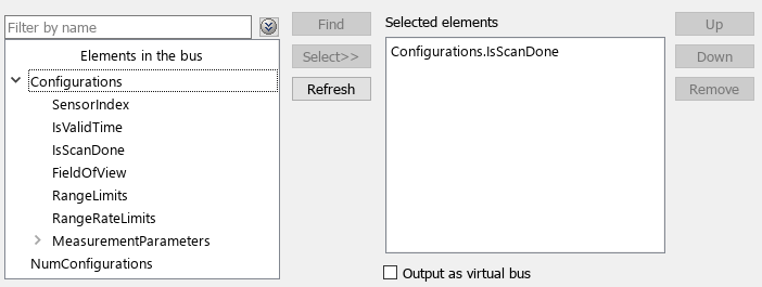
The radar sensor is modeled as a rotating radar which scans mechanically across the azimuth and elevation directions and completes a full scan within multiple updates. The IsScanDone bus element in the sensor configuration is returned as true when the sensor completes a full scan. You use the Bus Selector (Simulink) block to extract the IsScanDone element from the sensor configuration bus output.
Tracker
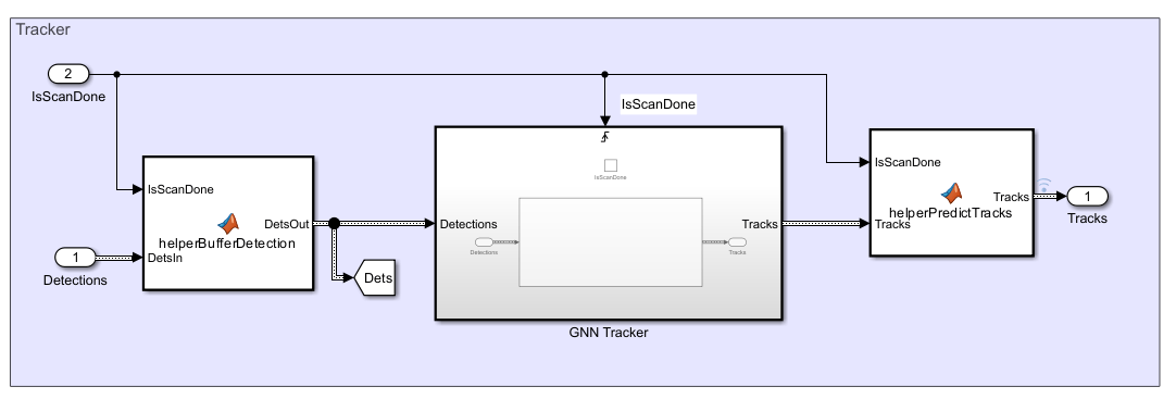
For each step in the scenario, the radar generates detections from targets in its field of view. After the radar completes a 360-degree scan in azimuth, the tracker updates with detections from the radar. Detections from the sensors are buffered until a full scan is complete. The buffer is implemented using a MATLAB Function (Simulink) block. When the IsScanDone flag is true, the buffer is released.
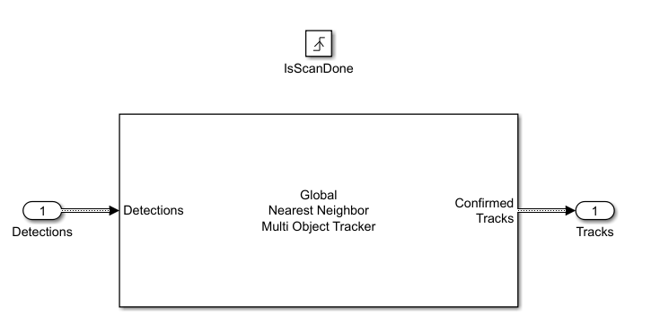
To ensure that the tracker only updates when a full sensor scan in complete, add a Global Nearest Neighbor Multi Object Tracker block in a Triggered Subsystem (Simulink) block. The block is triggered when isScanDone is true. When the full scan is not complete during the intermediate sensor updates, the tacks from previous time step are predicted to the current simulation time using a constvel motion model. The helperPredictTracks block is implemented using a MATLAB Function block.
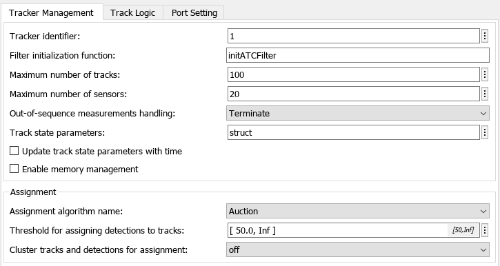

You configure the tracker block by setting the assignment algorithm to Auction, and threshold for assigning detection to tracks to 50. You also set the filter initialization function to initATCFilter, which initializes a constant velocity extended Kalman filter for each new track. See initATCFilter.m in the example folder for more details. You use the default confirmation and deletion thresholds to confirm and delete tracks, respectively. A confirmation threshold [2,3] means that a track is confirmed if a detection is assigned to it at least 2 times in the last 3 tracker updates and a deletion threshold [5,5] means that a confirmed track is deleted if any detection is not assigned to the track in the last 5 tracker updates.
Visualization
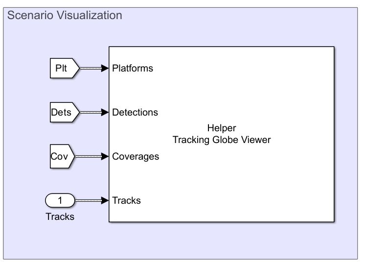
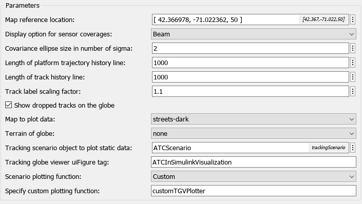
Implemented using the MATLAB System (Simulink) block, the Helper Tracking Globe Viewer block visualizes the scenario bases on the trackingGlobeViewer object. See the helperScenarioVisualization.m class in the example folder for the definition of the helper block.
Simulate and Track Airliners
Simulate the model and obtain the output.
simOut = sim(model);
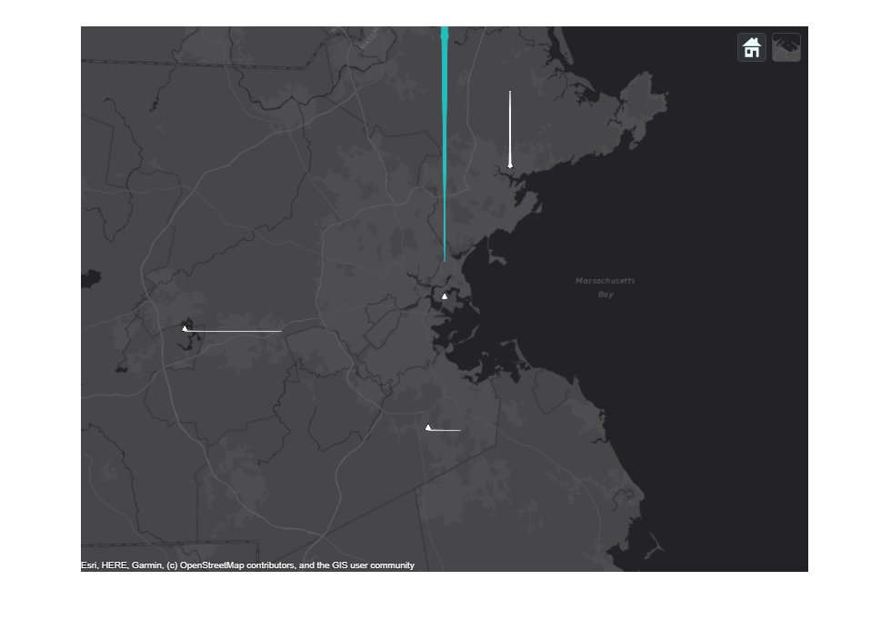
Show the first snapshot taken when the radar completes the second scan.
imshow(allsnaps{1})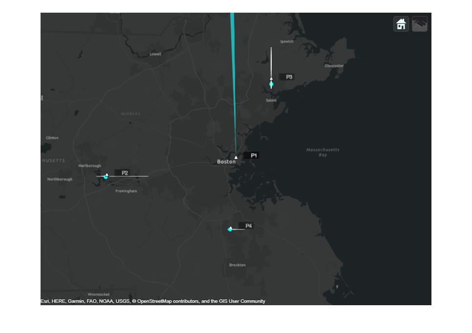
The figure above shows the scenario at the end of the second 360-degree scan of the radar. Radar detections, shown as light blue dots, are present for each of the simulated airliners. At this point, the tracker has already been updated by detections of one complete scan. Internally, the tracker has initialized tracks for each of the airliners. These tracks will be later confirmed and shown in the plot after more updates.
The next two snapshots show the tracking results for the outbound airliner.
imshow(allsnaps{2})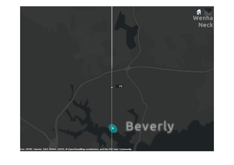
imshow(allsnaps{3})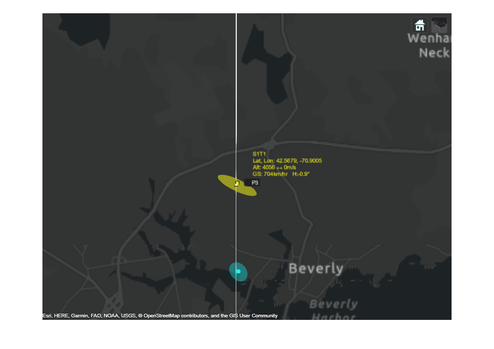
These two figures show the tracking results before and immediately after the tracker updates with the detections from second scan of the radar. The detection shown in the first figure is used to update and confirm the initialized track from the previous step. The next figure shows the confirmed track. The uncertainty of the track position estimate is shown as the yellow ellipse. After updating with only two detections, the tracker has established an accurate estimate of the outbound airliner. The true altitude of the airliner is 4 km traveling north at a speed of 700 km/hr.
imshow(allsnaps{4})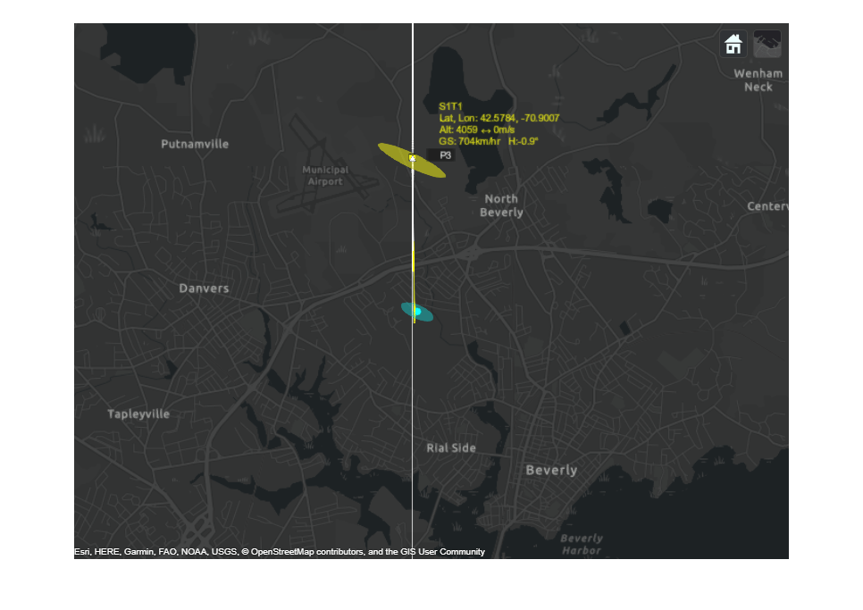
imshow(allsnaps{5})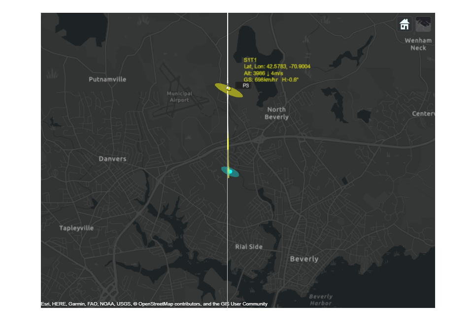
The track for the outbound airliner is coasted to the end of the third scan and shown in the figure above along with the most recent detection for the airliner. Notice how the track's uncertainty has grown since the last step. In the next figure, you can see the uncertainty of the track position is reduced after updating with the new detection. You also observe that after the third update, the track becomes closer to the airliner's true position.
imshow(allsnaps{6})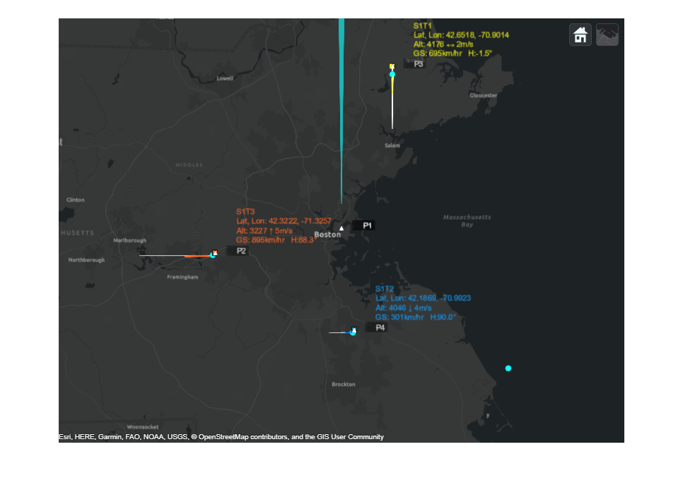
The final figure shows the state of all three tracks of the airliners at the end of the scenario. There is exactly one track for each airliner. The same track IDs are assigned to the airliners for the entire duration of the scenario, indicating that none of these tracks was dropped or switched during the scenario. The estimated tracks closely match the true position and velocity of the airliners.
disp(tabulateData(ATCScenario, simOut))
    TrackID        Altitude              Heading               Speed
               True    Estimated    True    Estimated    True    Estimated
    _______    _________________    _________________    _________________

     "T1"      4000      4040        90        91        700        695
     "T2"      4000      3964         0         0        300        301
     "T3"      3000      3126         0         2        900        895
close_system(model,0)
Summary
This example shows how to design a tracking system for an air traffic control center in Simulink and configure a global nearest neighbor (GNN) tracker block to track the simulated targets using the radar detections. In this example, you learned how the history-based logic promotes tracks. You also learned how the track uncertainty grows when a track is coasted and is reduced when the track is updated by a new detection.