Estimate Nonlinear ARX Models at the Command Line

You can estimate nonlinear ARX models after you perform the following tasks:

Prepare your data, as described in Preparing Data for Nonlinear Identification.
(Optional) Estimate model orders and delays the same way you would for linear ARX models. See Preliminary Step – Estimating Model Orders and Input Delays.
(Optional) Choose a mapping function for the output function in Available Mapping Functions for Nonlinear ARX Models.
(Optional) Estimate or construct a linear ARX model for initialization of nonlinear ARX model. See Initialize Nonlinear ARX Estimation Using Linear Model.

Estimate Model Using `nlarx`

Use nlarx to both construct and estimate a nonlinear ARX model. After each estimation, validate the model by comparing it to other models and simulating or predicting the model response.

Basic Estimation

Start with the simplest estimation using m = nlarx(data,[na nb nk]). For example:

load iddata1;
% na = nb = 2 and nk = 1 
m = nlarx(z1,[2 2 1])

m =

Nonlinear ARX model with 1 output and 1 input
  Inputs: u1
  Outputs: y1

Regressors:
  Linear regressors in variables y1, u1

Output function: Wavelet network with 1 units
Sample time: 0.1 seconds

Status:                                          
Estimated using NLARX on time domain data "z1".  
Fit to estimation data: 68.83% (prediction focus)
FPE: 1.975, MSE: 1.885                           
More information in model's "Report" property.

View the regressors.

getreg(m)

ans = 4x1 cell
    {'y1(t-1)'}
    {'y1(t-2)'}
    {'u1(t-1)'}
    {'u1(t-2)'}

The second input argument [na nb nk] specifies the model orders and delays. By default, the output function is the wavelet network idWaveletNetwork, which accepts regressors as inputs to its linear and nonlinear functions. m is an idnlarx object.

For MIMO systems, nb, nf, and nk are ny-by-nu matrices. See the nlarx reference page for more information about MIMO estimation.

Create an nlarxOptions option set and configure the Focus property to minimize simulation error.

opt = nlarxOptions('Focus','simulation');
M = nlarx(z1,[2 2 1],'idSigmoidNetwork',opt);

Configure Model Regressors

Linear Regressors

Linear regressors represent linear functions that are based on delayed input and output variables and which provide the inputs into the model output function. When you use orders to specify a model, the number of input regressors is equal to na and the number of output regressors is equal to nb. The orders syntax limits you to consecutive lags. You can also create linear regressors using linearRegressor. When you use linearRegressor, you can specify arbitrary lags.

Polynomial Regressors

Explore including polynomial regressors using polynomialRegressor in addition to the linear regressors in the nonlinear ARX model structure. Polynomial regressors are polynomial functions of delayed inputs and outputs. (see Nonlinear ARX Model Orders and Delay).

For example, generate polynomial regressors up to order 2.

P = polynomialRegressor({'y1','u1'},{[1],[2]},2);

Append the polynomial regressors to the linear regressors in m.Regressors.

m.Regressors = [m.Regressors;P];
getreg(m)

ans = 8x1 cell
    {'y1(t-1)'  }
    {'y1(t-2)'  }
    {'u1(t-1)'  }
    {'u1(t-2)'  }
    {'y1(t-3)'  }
    {'y1(t-5)'  }
    {'y1(t-1)^2'}
    {'u1(t-2)^2'}

m now includes polynomial regressors.

View the size of the m.Regressors array.

size(m.Regressors)

ans = 1×2

     3     1

The array now contains three regressor objects.

Custom Regressors

Use customRegressor to construct regressors as arbitrary functions of model input and output variables.

.For example, create two custom regressors that implement 'sin(y1(t-1)' and 'y1(t-2).*u1(t-3)'.

C1 = customRegressor({'y1'},{1},@(x)sin(x));
C2 = customRegressor({'y1','u1'},{2,3},@(x,y)x.*y);
m.Regressors = [m.Regressors;C1;C2];
getreg(m) % displays all regressors

ans = 10x1 cell
    {'y1(t-1)'         }
    {'y1(t-2)'         }
    {'u1(t-1)'         }
    {'u1(t-2)'         }
    {'y1(t-3)'         }
    {'y1(t-5)'         }
    {'y1(t-1)^2'       }
    {'u1(t-2)^2'       }
    {'sin(y1(t-1))'    }
    {'y1(t-2).*u1(t-3)'}

View the properties of custom regressors. For example, get the function handle of the first custom regressor in the array. This regressor is the fourth regressor set in the Regressors array.

C1_fcn = m.Regressors(4).VariablesToRegressorFcn

C1_fcn = function_handle with value:
    @(x)sin(x)

View the regressor description.

display(m.Regressors(4))

Custom regressor: sin(y1(t-1))
    VariablesToRegressorFcn: @(x)sin(x)
                  Variables: {'y1'}
                       Lags: {[1]}
                 Vectorized: 1
               TimeVariable: 't'

  Regressors described by this set

Combine Regressors

Once you have created linear, polynomial, and custom regressor objects, you can combine them in any way you want to suit your estimation needs.

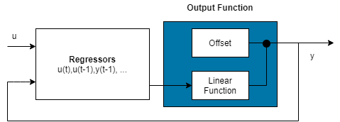
Specify Regressor Inputs to Linear and Nonlinear Components

Model regressors can enter as inputs to either or both linear and nonlinear function components of the mapping functions making up the output function. To reduce model complexity and keep the estimation well-conditioned, consider assigning a reduced set of regressors to the nonlinear component. You can also assign a subset of regressors to the linear component. The regressor usage table that manages the assignments provides complete flexibility. You can assign any combination of regressors to each component. For example, specify a nonlinear ARX model to be linear in past outputs and nonlinear in past inputs.

m = nlarx(z1,[2 2 1]); 
disp(m.RegressorUsage)

               y1:LinearFcn    y1:NonlinearFcn
               ____________    _______________

    y1(t-1)       true              true      
    y1(t-2)       true              true      
    u1(t-1)       true              true      
    u1(t-2)       true              true

m.RegressorUsage{3:4,1} = false;
m.RegressorUsage{1:2,2} = false;
disp(m.RegressorUsage)

               y1:LinearFcn    y1:NonlinearFcn
               ____________    _______________

    y1(t-1)       true              false     
    y1(t-2)       true              false     
    u1(t-1)       false             true      
    u1(t-2)       false             true

Configure Output Function

The following table summarizes available mapping objects for the model output function.

Mapping Description	Value (Default Mapping Object Configuration)	Mapping Object
Wavelet network (default)	`'idWaveletNetwork'` or `'wave'`	`idWaveletNetwork`
One layer sigmoid network	`'idSigmoidNetwork'` or `'sigm'`	`idSigmoidNetwork`
Tree partition	`'idTreePartition'` or `'tree'`	`idTreePartition`
F is linear in x	`'idLinear'` or `[ ]` or `''`	`idLinear`

Additional available mapping objects include multilayered neural networks and custom networks that you create.

Specify a multilayered neural network using:

m = nlarx(data,[na nb nk],NNet)

where NNet is the neural network object you create using the Deep Learning Toolbox™ software. See the idFeedforwardNetwork reference page.

Specify a custom network by defining a function called gaussunit.m, as described in the idCustomNetwork reference page. Define the custom network object CNetw and estimate the model:

CNetw = idCustomNetwork(@gaussunit);
m = nlarx(data,[na nb nk],CNetw)

Exclude Linear Function in Output Function

If your model output function includes idWaveletNetwork, idSigmoidNetwork, or idCustomNetwork mapping objects, you can exclude the linear function using the LinearFcn.Use property of the mapping object. The mapping object becomes F(x)= $g (Q (x - r)) + y_{0}$ , where g(.) is the nonlinear function and y₀ is the offset.

Note

You cannot exclude the linear function from tree partition and neural network mapping objects.

Exclude Nonlinear Function in Output Function

Configure the nonlinear ARX structure to include only the linear function in the mapping object by setting the mapping object to idLinear. In this case, $F (x) = L^{T} (x - r) + y_{0}$ is a weighted sum of model regressors plus an offset. Such models provide a bridge between purely linear ARX models and fully flexible nonlinear models.

A popular nonlinear ARX configuration in many applications uses polynomial regressors to model system nonlinearities. In such cases, the system is considered to be a linear combination of products of (delayed) input and output variables. Use the polynomialRegressor command to easily generate combinations of regressor products and powers.

For example, suppose that you know the output y(t) of a system to be a linear combination of (y(t − 1))², (u(t − 1))² and y(t − 1)u(t − 1)). To model such a system, use:

P = polynomialRegressor({'y1','u1'},{1,1},2)

P = 
Order 2 regressors in variables y1, u1
               Order: 2
           Variables: {'y1'  'u1'}
                Lags: {[1]  [1]}
         UseAbsolute: [0 0]
    AllowVariableMix: 0
         AllowLagMix: 0
        TimeVariable: 't'

  Regressors described by this set

P.AllowVariableMix = true;
M = nlarx(z1,P,idLinear);
getreg(M)

ans = 3x1 cell
    {'y1(t-1)^2'      }
    {'u1(t-1)^2'      }
    {'y1(t-1)*u1(t-1)'}

For more complex combinations of polynomial delays and mixed-variable regressors, you can also use customRegressor.

Iteratively Refine Model

If your model structure includes mapping objects that support iterative search (see Specify Estimation Options for Nonlinear ARX Models), you can use nlarx to refine model parameters:

m1 = nlarx(z1,[2 2 1],idSigmoidNetwork);
m2 = nlarx(z1,m1); % can repeatedly run this command

You can also use pem to refine the original model:

m2 = pem(z1,m1);

Check the search termination criterion m.Report.Termination.WhyStop . If WhyStop indicates that the estimation reached the maximum number of iterations, try repeating the estimation and possibly specifying a larger value for the nlarxOptions.SearchOptions.MaxIterations estimation option:

opt = nlarxOptions;
opt.SearchOptions.MaxIterations = 30;
m2 = nlarx(z1,m1,opt); % runs 30 more iterations
                               % starting from m1

When the m.Report.Termination.WhyStop value is Near (local) minimum, (norm( g) < tol or No improvement along the search direction with line search , validate your model to see if this model adequately fits the data. If not, the solution might be stuck in a local minimum of the cost-function surface. Try adjusting the SearchOptions.Tolerance value or the SearchMethod option in the nlarxOptions option set, and repeat the estimation.

You can also try perturbing the parameters of the last model using init (called randomization) and refining the model using nlarx:

M1 = nlarx(z1, [2 2 1], idSigmoidNetwork); % original model
M1p = init(M1);	% randomly perturbs parameters about nominal values
M2 = nlarx(z1, M1p);  % estimates parameters of perturbed model

You can display the progress of the iterative search in the MATLAB Command Window using the nlarxOptions.Display estimation option:

opt = nlarxOptions('Display','on');
M2= nlarx(z1,M1p,opt);

Troubleshoot Estimation

If you do not get a satisfactory model after many trials with various model structures and algorithm settings, it is possible that the data is poor. For example, your data might be missing important input or output variables and does not sufficiently cover all the operating points of the system.

Nonlinear black-box system identification usually requires more data than linear model identification to gain enough information about the system.

Use nlarx to Estimate Nonlinear ARX Models

Open Live Script

This example shows how to use nlarx to estimate a nonlinear ARX model for measured input/output data.

Prepare the data for estimation.

load twotankdata
z = iddata(y, u, 0.2);
ze = z(1:1000); zv = z(1001:3000);

Estimate several models using different model orders, delays, and nonlinearity settings.

m1 = nlarx(ze,[2 2 1]);
m2 = nlarx(ze,[2 2 3]);
m3 = nlarx(ze,[2 2 3],idWaveletNetwork(8));

An alternative way to perform the estimation is to configure the model structure first, and then to estimate this model.

m4 = idnlarx([2 2 3],idSigmoidNetwork(14));
m4.RegressorUsage.("y1:NonlinearFcn")(3:4) = false;
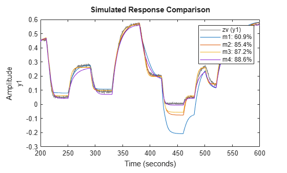
m4 = nlarx(ze,m4);

Compare the resulting models by plotting the model outputs with the measured output.

compare(zv, m1,m2,m3,m4)

Figure contains an axes object. The axes object with ylabel y1 contains 5 objects of type line. These objects represent Validation data (y1), m1: 60.91%, m2: 85.36%, m3: 87.16%, m4: 88.62%.