Estimate Nonlinear Grey-Box Models
Specifying the Nonlinear Grey-Box Model Structure
You must represent your system as a set of first-order nonlinear difference or differential equations:
where for continuous-time representation and for discrete-time representation with Ts as the sample time. F and H are arbitrary linear or nonlinear functions with Nx and Ny components, respectively. Nx is the number of states and Ny is the number of outputs.
After you establish the equations for your system, create a function or MEX file. MEX files, which can be created in C or Fortran, are dynamically linked subroutines that can be loaded and executed by the MATLAB®. For more information about MEX files, see Write C Functions Callable from MATLAB (MEX Files). This file is called an ODE file or a model file.
The purpose of the model file is to return the state derivatives and model outputs as a function of time, states, inputs, and model parameters, as follows:
[dx,y] = MODFILENAME(t,x,u,p1,p2,..,pN,FileArgument)
Tip
The template file for writing the C MEX file,
IDNLGREY_MODEL_TEMPLATE.c, is located in
matlab/toolbox/ident/nlident.
The output variables are:
dx— Represents the right side(s) of the state-space equation(s). A column vector with Nx entries. For static models,dx=[].For discrete-time models.
dxis the value of the states at the next time stepx(t+Ts).For continuous-time models.
dxis the state derivatives at time t, or .y— Represents the right side(s) of the output equation(s). A column vector with Ny entries.
The file inputs are:
t— Current time.x— State vector at timet. For static models, equals[].u— Input vector at timet. For time-series models, equals[].p1,p2, ...,pN— Parameters, which can be real scalars, column vectors or two-dimensional matrices.Nis the number of parameter objects. For scalar parameters,Nis the total number of parameter elements.FileArgument— Contains auxiliary variables that might be required for updating the constants in the state equations.
Tip
After creating a model file, call it directly from the MATLAB software with reasonable inputs and verify the output values. Also check that for the expected input and parameter value ranges, the model output and derivatives remain finite.
For an example of creating grey-box model files and idnlgrey model
object, see Creating idnlgrey Model
Files.
For examples of code files and MEX files that specify model structure, see the
toolbox/ident/iddemos/examples folder. For example, the model of a DC
motor is described in files dcmotor_m and
dcmotor_c.
Constructing the idnlgrey Object
After you create the function or MEX file with your model structure, define an idnlgrey object. This object shares many of the properties of the linear
idgrey model object.
Use the following general syntax to define the idnlgrey model
object:
m = idnlgrey('filename',Order,Parameters,InitialStates)The idnlgrey arguments are defined as follows:
'— Name of the function or MEX file storing the model structure. This file must be on the MATLAB path when you use this model object for model estimation, prediction, or simulation.filename'Order— Vector with three entries[Ny Nu Nx], specifying the number of model outputsNy, the number of inputsNu, and the number of statesNx.Parameters— Parameters, specified asstructarrays, cell arrays, or double arrays.InitialStates— Specified in the same way as parameters. Must be the fourth input to theidnlgreyconstructor.
You can also specify additional properties of the idnlgrey model,
including simulation method and related options. For detailed information about this object
and its properties, see the idnlgrey reference page.
Use nlgreyest or pem to estimate your grey-box model. Before estimating, it is advisable to
simulate the model to verify that the model file has been coded correctly. For example,
compute the model response to estimation data's input signal using sim:
y = sim(model,data)
model is the idnlgrey object, and
data is the estimation data (iddata object).Using nlgreyest to Estimate Nonlinear Grey-Box Models
You can use the nlgreyest command to estimate the unknown
idnlgrey model parameters and initial states
using measured data.
The input-output dimensions of the data must be compatible with the input and output
orders you specified for the idnlgrey model.
Use the following general estimation syntax:
m2 = nlgreyest(data,m)
where data is the estimation data and m is the
idnlgrey model object you constructed. The output
m2 is an idnlgrey model of same configuration as
m, with parameters and initial states updated to fit the data. More
information on estimation can be retrieved from the Report property. For
more information on Report and how to use it, see Output Arguments in the nlgreyest reference page, or type m2.Report on the command
line.
You can specify additional estimation options using the nlgreyestOptions option set, including SearchMethod and
SearchOption.
For information about validating your models, see Model Validation.
Represent Nonlinear Dynamics Using MATLAB File for Grey-Box Estimation
This example shows how to construct, estimate and analyze nonlinear grey-box models.
Nonlinear grey-box (idnlgrey) models are suitable for estimating parameters of systems that are described by nonlinear state-space structures in continuous or discrete time. You can use both idgrey (linear grey-box model) and idnlgrey objects to model linear systems. However, you can only use idnlgrey to represent nonlinear dynamics. To learn about linear grey-box modeling using idgrey, see Building Structured and User-Defined Models Using System Identification Toolbox.
About the Model
In this example, you model the dynamics of a linear DC motor using the idnlgrey object.
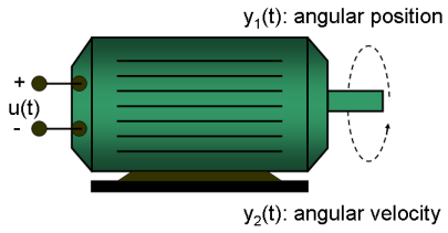
Figure 1: Schematic diagram of a DC-motor.
If you ignore the disturbances and choose y(1) as the angular position [rad] and y(2) as the angular velocity [rad/s] of the motor, you can set up a linear state-space structure of the following form (see Ljung, L. System Identification: Theory for the User, Upper Saddle River, NJ, Prentice-Hall PTR, 1999, 2nd ed., p. 95-97 for the derivation):
   d         | 0      1   |        |   0   |
   -- x(t) = |            | x(t) + |       | u(t)
   dt        | 0   -1/tau |        | k/tau |
             | 1   0 |
      y(t) = |       | x(t)
             | 0   1 |
tau is the time-constant of the motor in [s] and k is the static gain from the input to the angular velocity in [rad/(V*s)]. See Ljung (1999) for how tau and k relate to the physical parameters of the motor.
About the Input-Output Data
1. Load the DC motor data.
load('dcmotordata');
2. Represent the estimation data as an iddata object.
z = iddata(y, u, 0.1, 'Name', 'DC-motor');
3. Specify input and output signal names, start time and time units.
z.InputName = 'Voltage';
z.InputUnit =  'V';
z.OutputName = {'Angular position', 'Angular velocity'};
z.OutputUnit = {'rad', 'rad/s'};
z.Tstart = 0;
z.TimeUnit = 's';
4. Plot the data.
The data is shown in two plot windows.
figure('Name', [z.Name ': Voltage input -> Angular position output']);
plot(z(:, 1, 1));   % Plot first input-output pair (Voltage -> Angular position).
figure('Name', [z.Name ': Voltage input -> Angular velocity output']);
plot(z(:, 2, 1));   % Plot second input-output pair (Voltage -> Angular velocity).
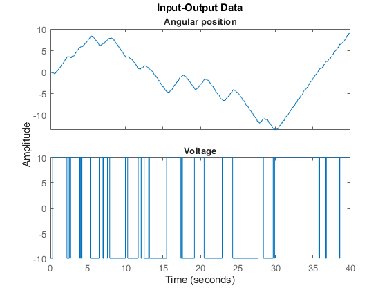
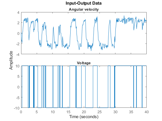
Figure 2: Input-output data from a DC-motor.
Linear Modeling of the DC-Motor
1. Represent the DC motor structure in a function.
In this example, you use a MATLAB® file, but you can also use C MEX-files (to gain computational speed), P-files or function handles. For more information, see Creating IDNLGREY Model Files.
The DC-motor function is called dcmotor_m.m and is shown below.
function [dx, y] = dcmotor_m(t, x, u, tau, k, varargin)
  % Output equations.
  y = [x(1);                         ... % Angular position.
       x(2)                          ... % Angular velocity.
      ];
% State equations.
dx = [x(2); ... % Angular velocity.
-(1/tau)*x(2)+(k/tau)*u(1) ... % Angular acceleration.
];The file must always be structured to return the following:
Output arguments:
dxis the vector of state derivatives in continuous-time case, and state update values in the discrete-time case.
yis the output equation
Input arguments:
The first three input arguments must be:
t(time),x(state vector, [] for static systems),u(input vector, [] for time-series).
Ordered list of parameters follow. The parameters can be scalars, column vectors, or 2-dimensional matrices.
vararginfor the auxiliary input arguments
2. Represent the DC motor dynamics using an idnlgrey object.
The model describes how the inputs generate the outputs using the state equation(s).
FileName      = 'dcmotor_m';       % File describing the model structure.
Order         = [2 1 2];           % Model orders [ny nu nx].
Parameters    = [1; 0.28];         % Initial parameters. Np = 2.
InitialStates = [0; 0];            % Initial initial states.
Ts            = 0;                 % Time-continuous system.
nlgr = idnlgrey(FileName, Order, Parameters, InitialStates, Ts, ...
                'Name', 'DC-motor');
In practice, there are disturbances that affect the outputs. An idnlgrey model does not explicitly model the disturbances, but assumes that these are just added to the output(s). Thus, idnlgrey models are equivalent to Output-Error (OE) models. Without a noise model, past outputs do not influence prediction of future outputs, which means that predicted output for any prediction horizon k coincide with simulated outputs.
3. Specify input and output names, and units.
set(nlgr, 'InputName', 'Voltage', 'InputUnit', 'V',               ...
          'OutputName', {'Angular position', 'Angular velocity'}, ...
          'OutputUnit', {'rad', 'rad/s'},                         ...
          'TimeUnit', 's');
4. Specify names and units of the initial states and parameters.
nlgr = setinit(nlgr, 'Name', {'Angular position' 'Angular velocity'});
nlgr = setinit(nlgr, 'Unit', {'rad' 'rad/s'});
nlgr = setpar(nlgr, 'Name', {'Time-constant' 'Static gain'});
nlgr = setpar(nlgr, 'Unit', {'s' 'rad/(V*s)'});
You can also use setinit and setpar to assign values, minima, maxima, and estimation status for all initial states or parameters simultaneously.
5. View the initial model.
a. Get basic information about the model.
The DC-motor has 2 (initial) states and 2 model parameters.
size(nlgr)
Nonlinear grey-box model with 2 outputs, 1 inputs, 2 states and 2 parameters (2 free).
b. View the initial states and parameters.
Both the initial states and parameters are structure arrays. The fields specify the properties of an individual initial state or parameter. Type help idnlgrey.InitialStates and help idnlgrey.Parameters for more information.
nlgr.InitialStates(1)
nlgr.Parameters(2)
ans =

  struct with fields:

       Name: 'Angular position'
       Unit: 'rad'
      Value: 0
    Minimum: -Inf
    Maximum: Inf
      Fixed: 1


ans =

  struct with fields:

       Name: 'Static gain'
       Unit: 'rad/(V*s)'
      Value: 0.2800
    Minimum: -Inf
    Maximum: Inf
      Fixed: 0
c. Retrieve information for all initial states or model parameters in one call.
For example, obtain information on initial states that are fixed (not estimated) and the minima of all model parameters.
getinit(nlgr, 'Fixed')
getpar(nlgr, 'Min')
ans =

  2×1 cell array

    {[1]}
    {[1]}


ans =

  2×1 cell array

    {[-Inf]}
    {[-Inf]}
d. Obtain basic information about the object:
nlgr
nlgr =

Continuous-time nonlinear grey-box model defined by 'dcmotor_m' (MATLAB file):

   dx/dt = F(t, x(t), u(t), p1, p2)
    y(t) = H(t, x(t), u(t), p1, p2) + e(t)

 with 1 input(s), 2 state(s), 2 output(s), and 2 free parameter(s) (out of 2).

Name: DC-motor

Status:
Created by direct construction or transformation. Not estimated.
Use get to obtain more information about the model properties. The idnlgrey object shares many properties of parametric linear model objects.
get(nlgr)
             FileName: 'dcmotor_m'
                Order: [1×1 struct]
           Parameters: [2×1 struct]
        InitialStates: [2×1 struct]
         FileArgument: {}
    SimulationOptions: [1×1 struct]
         TimeVariable: 't'
        NoiseVariance: [2×2 double]
            InputName: {'Voltage'}
            InputUnit: {'V'}
           InputGroup: [1×1 struct]
           OutputName: {2×1 cell}
           OutputUnit: {2×1 cell}
          OutputGroup: [1×1 struct]
                Notes: [0×1 string]
             UserData: []
                 Name: 'DC-motor'
                   Ts: 0
             TimeUnit: 'seconds'
               Report: [1×1 idresults.nlgreyest]
Performance Evaluation of the Initial DC-Motor Model
Before estimating the parameters tau and k, simulate the output of the system with the parameter guesses using the default differential equation solver (a Runge-Kutta 45 solver with adaptive step length adjustment). The simulation options are specified using the "SimulationOptions" model property.
1. Set the absolute and relative error tolerances to small values (1e-6 and 1e-5, respectively).
nlgr.SimulationOptions.AbsTol = 1e-6;
nlgr.SimulationOptions.RelTol = 1e-5;
2. Compare the simulated output with the measured data.
compare displays both measured and simulated outputs of one or more models, whereas predict, called with the same input arguments, displays the simulated outputs.
The simulated and measured outputs are shown in a plot window.
compare(z, nlgr);
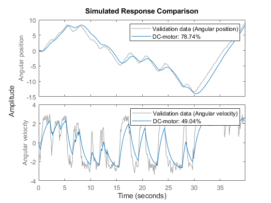
Figure 3: Comparison between measured outputs and the simulated outputs of the initial DC-motor model.
Parameter Estimation
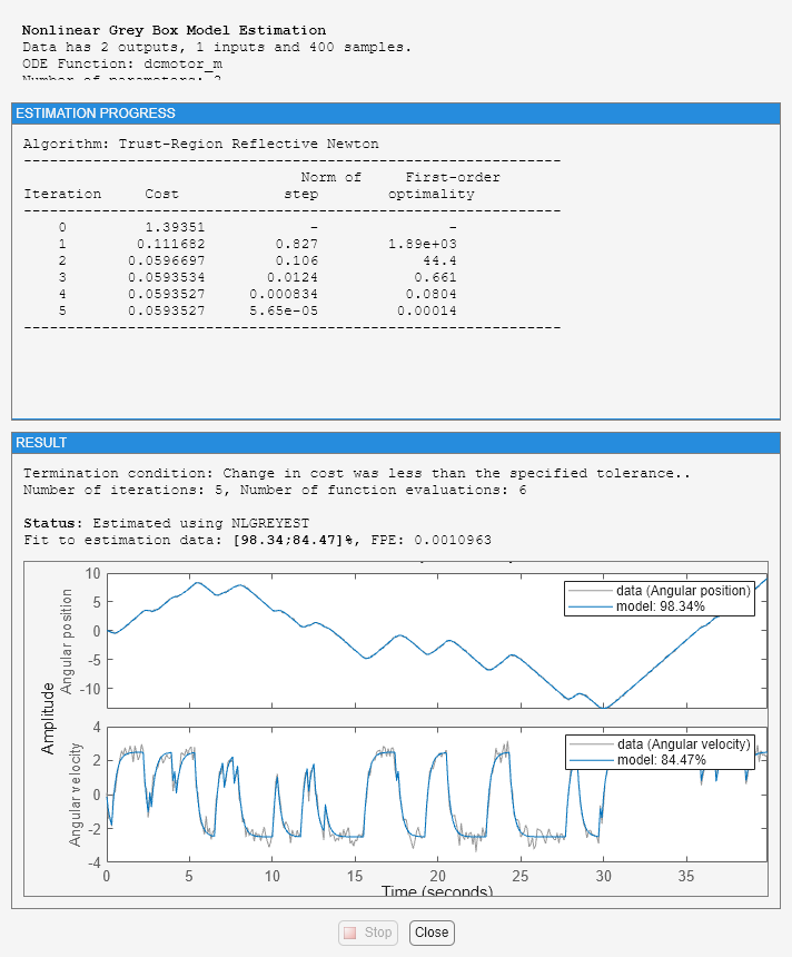
Estimate the parameters and initial states using nlgreyest, which is a prediction error minimization method for nonlinear grey box models. The estimation options, such as the choice of estimation progress display, are specified using the "nlgreyestOptions" option set.
nlgr = setinit(nlgr, 'Fixed', {false false}); % Estimate the initial states.
opt = nlgreyestOptions('Display', 'on');
nlgr = nlgreyest(z, nlgr, opt);
Performance Evaluation of the Estimated DC-Motor Model
1. Review the information about the estimation process.
This information is stored in the Report property of the idnlgrey object. The property also contains information about how the model was estimated, such as solver and search method, data set, and why the estimation was terminated.
nlgr.Report
fprintf('\n\nThe search termination condition:\n')
nlgr.Report.Termination
ans =

         Status: 'Estimated using NLGREYEST'
         Method: 'Solver: ode45; Search: lsqnonlin'
            Fit: [1×1 struct]
     Parameters: [1×1 struct]
    OptionsUsed: [1×1 idoptions.nlgreyest]
      RandState: []
       DataUsed: [1×1 struct]
    Termination: [1×1 struct]


The search termination condition:

ans =

  struct with fields:

                 WhyStop: 'Change in cost was less than the specified tolerance.'
              Iterations: 5
    FirstOrderOptimality: 1.4014e-04
                FcnCount: 6
               Algorithm: 'trust-region-reflective'
2. Evaluate the model quality by comparing simulated and measured outputs.
The fits are 98% and 84%, which indicate that the estimated model captures the dynamics of the DC motor well.
compare(z, nlgr);
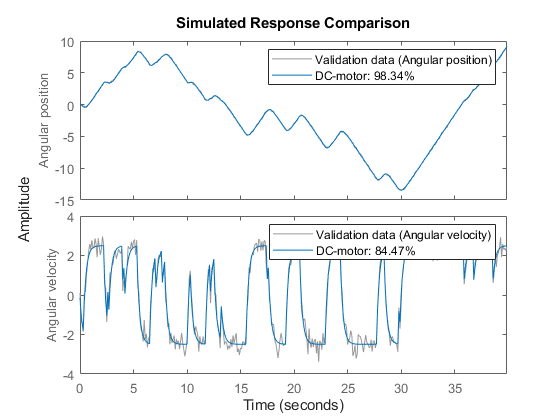
Figure 4: Comparison between measured outputs and the simulated outputs of the estimated IDNLGREY DC-motor model.
3. Compare the performance of the idnlgrey model with a second-order ARX model.
na = [2 2; 2 2];
nb = [2; 2];
nk = [1; 1];
dcarx = arx(z, [na nb nk]);
compare(z, nlgr, dcarx);
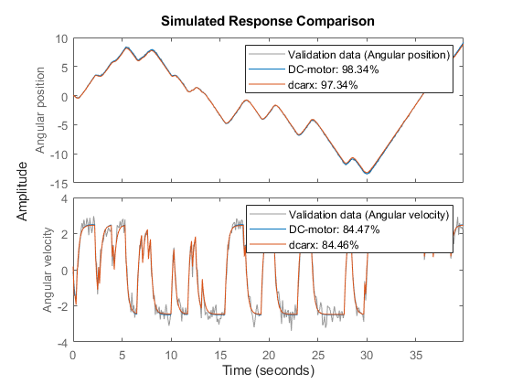
Figure 5: Comparison between measured outputs and the simulated outputs of the estimated IDNLGREY and ARX DC-motor models.
4. Check the prediction errors.
The prediction errors obtained are small and are centered around zero (non-biased).
pe(z, nlgr);
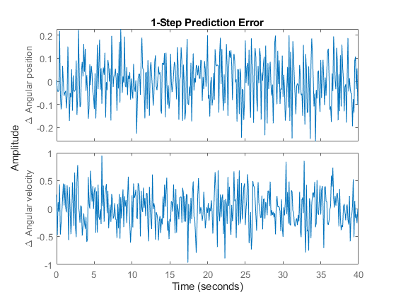
Figure 6: Prediction errors obtained with the estimated IDNLGREY DC-motor model.
5. Check the residuals ("leftovers").
Residuals indicate what is left unexplained by the model and are small for good model quality. Use the resid command to view the correlations among the residuals. The first column of plots shows the autocorrelations of the residuals for the two outputs. The second column shows the cross-correlation of these residuals with the input "Voltage". The correlations are within acceptable bounds (blue region).
figure('Name',[nlgr.Name ': residuals of estimated model']);
resid(z,nlgr);
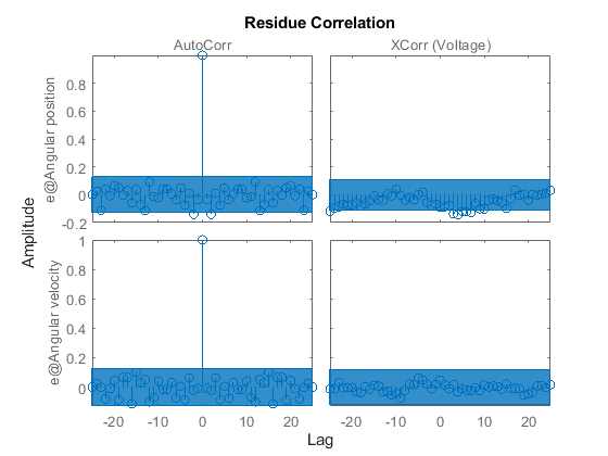
Figure 7: Residuals obtained with the estimated IDNLGREY DC-motor model.
6. Plot the step response.
A unit input step results in an angular position showing a ramp-type behavior and to an angular velocity that stabilizes at a constant level.
figure('Name', [nlgr.Name ': step response of estimated model']);
step(nlgr);
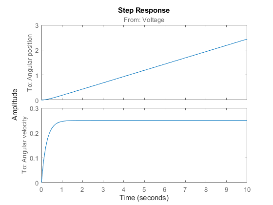
Figure 8: Step response with the estimated IDNLGREY DC-motor model.
7. Examine the model covariance.
You can assess the quality of the estimated model to some extent by looking at the estimated covariance matrix and the estimated noise variance. A "small" value of the (i, i) diagonal element of the covariance matrix indicates that the i:th model parameter is important for explaining the system dynamics when using the chosen model structure. Small noise variance (covariance for multi-output systems) elements are also a good indication that the model captures the estimation data in a good way.
getcov(nlgr)
nlgr.NoiseVariance
ans =

   1.0e-04 *

    0.1573    0.0021
    0.0021    0.0008


ans =

    0.0010   -0.0000
   -0.0000    0.0110
For more information about the estimated model, use present to display the initial states and estimated parameter values, and estimated uncertainty (standard deviation) for the parameters.
present(nlgr);
nlgr =

Continuous-time nonlinear grey-box model defined by 'dcmotor_m' (MATLAB file):

   dx/dt = F(t, x(t), u(t), p1, p2)
    y(t) = H(t, x(t), u(t), p1, p2) + e(t)

 with 1 input(s), 2 state(s), 2 output(s), and 2 free parameter(s) (out of 2).

 Inputs:
    u(1)  Voltage(t) [V]
 States:                              Initial value
    x(1)  Angular position(t) [rad]     xinit@exp1   0.0302675   (estimated) in [-Inf, Inf]
    x(2)  Angular velocity(t) [rad/s]   xinit@exp1   -0.133777   (estimated) in [-Inf, Inf]
 Outputs:
    y(1)  Angular position(t) [rad]
    y(2)  Angular velocity(t) [rad/s]
 Parameters:                        Value Standard Deviation
    p1   Time-constant [s]           0.243649       0.00396671   (estimated) in [-Inf, Inf]
    p2   Static gain [rad/(V*s)]     0.249644      0.000284486   (estimated) in [-Inf, Inf]

Name: DC-motor

Status:
Termination condition: Change in cost was less than the specified tolerance..
Number of iterations: 5, Number of function evaluations: 6

Estimated using Solver: ode45; Search: lsqnonlin on time domain data "DC-motor".
Fit to estimation data: [98.34;84.47]%
FPE: 0.001096, MSE: 0.1187
More information in model's "Report" property.
Conclusions
This example illustrates the basic tools for performing nonlinear grey-box modeling. See the other nonlinear grey-box examples to learn about:
Using nonlinear grey-box models in more advanced modeling situations, such as building nonlinear continuous- and discrete-time, time-series and static models.
Writing and using C MEX model-files.
Handling nonscalar parameters.
Impact of certain algorithm choices.
For more information on identification of dynamic systems with System Identification Toolbox™, visit the System Identification Toolbox product information page.
Nonlinear Grey-Box Model Properties and Estimation Options
idnlgrey creates a nonlinear grey-box model based on the model
structure and properties. The parameters and initial states of the created
idnlgrey object are estimated using nlgreyest.
The following model properties and estimation options affect the model creation and estimation results.
Simulation Method
You specify the simulation method using the SimulationOptions
(struct) property of idnlgrey.
System Identification Toolbox™ software provides several variable-step and fixed-step solvers for
simulating idnlgrey models.
For discrete-time systems, the default solver is
'FixedStepDiscrete'. For continuous-time systems, the default solver
is 'ode45'. By default, SimulationOptions.Solver is
set to 'Auto', which automatically selects either
'ode45' or 'FixedStepDiscrete' during estimation
and simulation—depending on whether the system is continuous or discrete in
time.
To view a list of available solvers and their properties, see the
SimulationOptions model property in idnlgrey reference page.
Search Method
You specify the search method for estimating model parameters using the
SearchMethod option of the nlgreyestOptions
option set. Two categories of methods are available for nonlinear grey-box
modeling.
One category of methods consists of the minimization schemes that are based on line-search methods, including Gauss-Newton type methods, steepest-descent methods, and Levenberg-Marquardt methods.
The Trust-Region Reflective Newton method of nonlinear least-squares
(lsqnonlin), where the cost is the sum of squares of errors between
the measured and simulated outputs, requires Optimization Toolbox™ software. When the parameter bounds differ from the default +/- Inf, this
search method handles the bounds better than the schemes based on a line search. However,
unlike the line-search-based methods, lsqnonlin cannot handle automatic
weighting by the inverse of estimated noise variance in multi-output cases. For more
information, see OutputWeight estimation option in the nlgreyestOptions reference page.
By default, SearchMethod is set to Auto, which
automatically selects a method from the available minimizers. If the Optimization Toolbox product is installed, SearchMethod is set to
'lsqnonlin'. Otherwise, SearchMethod is a
combination of line-search based schemes.
For detailed information about this and other nlgreyest
estimation options, see nlgreyestOptions.
Gradient Options
You specify the method for calculating gradients using the
GradientOptions option of the nlgreyestOptions
option set. Gradients are the derivatives of errors with respect to
unknown parameters and initial states.
Gradients are calculated by numerically perturbing unknown quantities and measuring their effects on the simulation error.
Option for gradient computation include the choice of the differencing scheme (forward, backward or central), the size of minimum perturbation of the unknown quantities, and whether the gradients are calculated simultaneously or individually.
For detailed information about this and other nlgreyest
estimation options, see nlgreyestOptions.