Estimate Linear Grey-Box Models

Specifying the Linear Grey-Box Model Structure

You can estimate linear discrete-time and continuous-time grey-box models for arbitrary ordinary differential or difference equations using single-output and multiple-output time-domain data, or time-series data (output-only).

You must represent your system equations in state-space form. State-space models use state variables x(t) to describe a system as a set of first-order differential equations, rather than by one or more nth-order differential equations.

The first step in grey-box modeling is to write a function that returns state-space matrices as a function of user-defined parameters and information about the model.

Use the following format to implement the linear grey-box model in the file:

[A,B,C,D] = myfunc(par1,par2,...,parN,Ts,aux1,aux2,...)

where the output arguments are the state-space matrices and myfunc is the name of the file. par1,par2,...,parN are the N parameters of the model. Each entry may be a scalar, vector or matrix.Ts is the sample time. aux1,aux2,... are the optional input arguments that myfunc uses to compute the state-space matrices in addition to the parameters and sample time. aux contains auxiliary variables in your system. You use auxiliary variables to vary system parameters at the input to the function, and avoid editing the file.

You can write the contents of myfunc to parameterize either a continuous-time, or a discrete-time state-space model, or both. When you create the linear grey-box model using myfunc, you can specify the nature of the output arguments of myfunc. The continuous-time state-space model has the form:

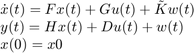
In continuous-time, the state-space description has the following form:

$$\begin{array}{l}\dot{x}(t)=Ax(t)+Bu(t)+Ke(t)\\ y(t)=Cx(t)+Du(t)+e(t)\\ x(0)=x0\end{array}$$

where, A,B,C and D are matrices that are parameterized by the parameters par1,par2,...,parN. The noise matrix K and initial state vector, x0, are not parameterized by myfunc. In some applications, you may want to express K and x0 as quantities that are parameterized by chosen parameters, just as the A, B, C and D matrices. To handle such cases, you can write the ODE file, myfunc, to return K and x0 as additional output arguments:

[A,B,C,D,K,x0] = myfunc(par1,par2,...,parN,Ts,aux1,aux2,...)

K and x0 are thus treated in the same way as the A, B, C and D matrices. They are all functions of the parameters par1,par2,...,parN. To configure the handling of initial states, x0, and the disturbance component, K, during estimation, use the greyestOptions option set.

In discrete-time, the state-space description has a similar form:

$$\begin{array}{l}x(k+1)=Ax(k)+Bu(k)+Ke(t)\\ y(k)=Cx(k)+Du(k)+e(t)\\ x(0)=x0\end{array}$$

where, A, B, C and D are now the discrete-time matrices that are parameterized by the parameters par1,par2,...,parN. K and x0 are not directly parameterized, but can be estimated if required by configuring the corresponding estimation options.

After creating the function or MEX-file with your model structure, you must define an idgrey model object.

Create Function to Represent a Grey-Box Model

This example shows how to represent the structure of the following continuous-time model:

This equation represents an electrical motor, where is the angular position of the motor shaft, and is the angular velocity. The parameter is the inverse time constant of the motor, and is the static gain from the input to the angular velocity.

The motor is at rest at t = 0, but its angular position is unknown. Suppose that the approximate nominal values of the unknown parameters are , and . For more information about this example, see the section on state-space models in System Identification: Theory for the User , Second Edition, by Lennart Ljung, Prentice Hall PTR, 1999.

The continuous-time state-space model structure is defined by the following equation:

If you want to estimate the same model using a structured state-space representation, see Estimate Structured Continuous-Time State-Space Models.

To prepare this model for estimation:

• Create the following file to represent the model structure in this example:

function [A,B,C,D,K,x0] = myfunc(par,T)
A = [0 1; 0 par(1)]; 
B = [0;par(2)];
C = eye(2);
D = zeros(2,1);
K = zeros(2,2);
x0 = [par(3);0];

Save the file such that it is in the MATLAB® search path.

• Use the following syntax to define an idgrey model object based on the myfunc file:

par = [-1; 0.25; 0];
aux = {};
T = 0;
m = idgrey('myfunc',par,'c',aux,T);

where par represents a vector of all the user-defined parameters and contains their nominal (initial) values. In this example, all the scalar-valued parameters are grouped in the par vector. The scalar-valued parameters could also have been treated as independent input arguments to the ODE function myfunc. 'c' specifies that the underlying parameterization is in continuous time. aux represents optional arguments. As myfunc does not have any optional arguments, use aux = {}. T specifies the sample time; T = 0 indicates a continuous-time model.

Load the estimation data.

load dcmotordata
data = iddata(y,u,0.1);

Use greyest to estimate the grey-box parameter values:

m_est = greyest(data,m);

where data is the estimation data and m is an estimation initialization idgrey model. m_est is the estimated idgrey model.