About Identified Linear Models
What Are IDLTI Models?
System Identification Toolbox™ software uses objects to represent a variety of linear and nonlinear model structures. These linear model objects are collectively known as Identified Linear Time-Invariant (IDLTI) models.
IDLTI models contain two distinct dynamic components:
Measured component — Describes the relationship between the measured inputs and the measured output (G)
Noise component — Describes the relationship between the disturbances at the output and the measured output (H)
Models that only have the noise component H are called time-series or
signal models. Typically, you create such models using time-series data that consist of one or
more outputs y(t) with no corresponding input.
The total output is the sum of the contributions from the measured inputs and the disturbances: y = G u + H e, where u represents the measured inputs and e the disturbance. e(t) is modeled as zero-mean Gaussian white noise with variance Λ. The following figure illustrates an IDLTI model.
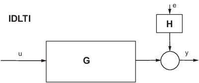
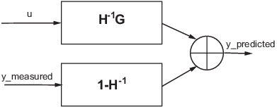
When you simulate an IDLTI model, you study the effect of input u(t) (and possibly initial conditions) on the output y(t). The noise e(t) is not considered. However, with finite-horizon prediction of the output, both the measured and the noise components of the model contribute towards computation of the (predicted) response.
One-step ahead prediction model corresponding to a linear identified model (y = Gu+He)
Measured and Noise Component Parameterizations
The various linear model structures provide different ways of parameterizing the transfer
functions G and H. When you construct an IDLTI model or
estimate a model directly using input-output data, you can configure the structure of both
G and H, as described in the following table:
| Model Type | Transfer Functions G and H | Configuration Method |
|---|---|---|
State space model (idss) |
Represents an identified state-space model structure, governed by the equations:
where the transfer function between the measured input u and output y is and the noise transfer function is . |
Construction: Use Estimation: Use |
Polynomial model (idpoly) |
Represents a polynomial model such as ARX, ARMAX and BJ. An ARMAX model, for example, uses the input-output equation Ay(t) = Bu(t)+Ce(t), so that the measured transfer function G is , while the noise transfer function is . The ARMAX model is a special configuration of the general polynomial model whose governing equation is: The autoregressive component, A, is common between the measured and noise components. The polynomials B and F constitute the measured component while the polynomials C and D constitute the noise component. |
Construction: Use y = idpoly([],B,[],[],F) Estimation: Use the |
Transfer function model (idtf) |
Represents an identified transfer function model, which has no dynamic elements to model noise behavior. This object uses the trivial noise model H(s) = I. The governing equation is
|
Construction: Use Estimation: Use |
Process model (idproc) |
Represents a process model, which provides options to represent the noise dynamics as either first- or second-order ARMA process (that is, H(s)= C(s)/A(s), where C(s) and A(s) are monic polynomials of equal degree). The measured component, G(s), is represented by a transfer function expressed in pole-zero form. |
For process (and grey-box) models, the noise component is often treated as an
on-demand extension to an otherwise measured component-centric representation. For these
models, you can add a noise component by using the model = procest(data,'P1D') estimates a model whose equation is:
To add a second order noise component to the model, use: Options = procestOptions('DisturbanceModel','ARMA1');
model = procest(data,'P1D',Options);
This model has the equation: where the coefficients c1 and d1 parameterize
the noise component of the model. If you are constructing a process model using the
model = idproc('P1','Kp',1,'Tp1',1,'NoiseTF',...
struct('num',[1 0.1],'den',[1 0.5]))
creates the process model y(s) = 1/(s+1) u(s) + (s + 0.1)/(s + 0.5) e(s) |
Sometimes, fixing coefficients or specifying bounds on the parameters are not sufficient.
For example, you may have unrelated parameter dependencies in the model or parameters may be a
function of a different set of parameters that you want to identify exclusively. For example, in
a mass-spring-damper system, the A and B parameters both
depend on the mass of the system. To achieve such parameterization of linear models, you can use
grey-box modeling where you establish the link between the actual parameters and model
coefficients by writing an ODE file. To learn more, see Grey-Box Model Estimation.
Linear Model Estimation
You typically use estimation to create models in System Identification Toolbox. You execute one of the estimation commands, specifying as input arguments the
measured data, along with other inputs necessary to define the structure of a model. To
illustrate, the following example uses the state-space estimation command, ssest, to create a state space model. The first input argument
data specifies the measured input-output data. The second input argument
specifies the order of the model.
sys = ssest(data,4)
The estimation function treats the noise variable e(t) as prediction error – the residual portion of the output that cannot be attributed to the measured inputs. All estimation algorithms work to minimize a weighted norm of e(t) over the span of available measurements. The weighting function is defined by the nature of the noise transfer function H and the focus of estimation, such as simulation or prediction error minimization.
Black Box (“Cold Start”) Estimation
In a black-box estimation, you only have to specify the order to configure the structure of the model.
sys = estimator(data,orders)
where estimator is the name of an estimation command to use for
the desired model type.
For example, you use tfest to estimate transfer function models,
arx for ARX-structure polynomial models, and procest for process models.
The first argument, data, is time- or frequency domain data represented
as an iddata or idfrd object. The second argument, orders, represents one or
more numbers whose definitions depends upon the model type:
For transfer functions,
ordersrefers to the number of poles and zeros.For state-space models,
ordersrefers to the number of states.For process models,
ordersdenotes the structural elements of a process model, such as, the number of poles and presence of delay and integrator.
When working with the app, you specify the orders in the appropriate edit fields of corresponding model estimation dialogs.
Structured Estimations
In some situations, you want to configure the structure of the desired model more closely
than what is achieved by simply specifying the orders. In such cases, you construct a template
model and configure its properties. You then pass that template model as an input argument to
the estimation commands in place of orders.
To illustrate, the following example assigns initial guess values to the numerator and the denominator polynomials of a transfer function model, imposes minimum and maximum bounds on their estimated values, and then passes the object to the estimator function.
% Initial guess for numerator
num = [1 2];
den = [1 2 1 1];
% Initial guess for the denominator
sys = idtf(num,den);
% Set min bound on den coefficients to 0.1
sys.Structure.Denominator.Minimum = [1 0.1 0.1 0.1];
sysEstimated = tfest(data,sys);
The estimation algorithm uses the provided initial guesses to kick-start the estimation and delivers a model that respects the specified bounds.
You can use such a model template to also configure auxiliary model properties such as
input/output names and units. If the values of some of the model’s parameters are initially
unknown, you can use NaNs for them in the template.
Estimation Options
There are many options associated with a model’s estimation algorithm that configure the
estimation objective function, initial conditions and numerical search algorithm, among other
things. For every estimation command, estimator, there is a
corresponding option command named
estimatorOptions. To specify options for a
particular estimator command, such as tfest, use the options command that
corresponds to the estimation command, in this case, tfestOptions. The
options command returns an options set that you then pass as an input argument to the
corresponding estimation command.
For example, to estimate an Output-Error structure polynomial model, you use oe. To specify simulation as the focus and
lsqnonlin as the search method, you use oeOptions:
load iddata1 z1
Options = oeOptions('Focus','simulation','SearchMethod','lsqnonlin');
sys= oe(z1,[2 2 1],Options);
Information about the options used to create an estimated model is stored in the
OptionsUsed field of the model’s Report property. For
more information, see Estimation Report.
More About Linear System Identification
For more information about linear system identification, play the video. This video is part of the System Identification video series.