Main Content

tfest

Estimate transfer function model

Description

Estimate Transfer Function Model

example

sys = tfest(tt,np) estimates the continuous-time transfer function sys with np poles, using all the input and output signals in the timetable tt. The number of zeros in sys is max(np-1,0). You can use this syntax for SISO and MISO systems. The function assumes that the last variable in the timetable is the single output signal.

You cannot use tfest to estimate time-series models, which are models that contain no inputs. Use ar, arx, or armax for time-series models instead.

example

sys = tfest(u,y,np) estimates a continuous-time transfer function using the time-domain input signals and output signals in the matrices u,y. The software assumes that the data sample time is 1 second. You cannot change this assumed sample time. If you want to estimate a model from data with a sample time other than 1 second, you have two alternatives:

  1. Estimate a discrete-time system instead by setting the sample time using the 'Ts' name-value argument. For example, sys = tfest(u,y,np,'Ts',0.1) sets the sample time to 0.1. You can use this syntax with SISO, MISO, and MIMO systems.

  2. Convert your matrix data to a timetable or iddata object prior to estimating a continuous-time system. These formats allow you to incorporate sample-time knowledge into the data. For more information, see u,y.

Estimating continuous-time models from matrix-based data is not recommended.

sys = tfest(data,np) uses the time-domain or frequency-domain data in data. Use this syntax especially when you want to estimate a transfer function using frequency-domain or frequency response data, or when you want to take advantage of the additional information, such as intersample behavior, data sample time, or experiment labeling, that data objects provide.

example

sys = tfest(___,nz) specifies the number of zeros nz. You can use this syntax with any of the previous input-argument combinations.

example

sys = tfest(___,nz,iodelay) specifies the transport delays iodelay for the input/output pairs.

example

sys = tfest(___,Name,Value) uses additional model options specified by one or more name-value pair arguments. For example, specify a discrete-time system from matrix data that has a sample time of 0.1 using sys = tfest(um,ym,np,'Ts',0.1). Specify input and output signal variable names that correspond with the variables to use for MIMO timetable data using sys = tfest(data,np,nz,'InputNames',["u1","u2"],'OutputNames',["y1","y3"]).

Configure Initial Parameters

sys = tfest(tt,init_sys) uses the linear system init_sys to configure the initial parameterization of sys for estimation using the timetable tt.

sys = tfest(u,y,init_sys) uses matrix data u,y for estimation. If init_sys is a continuous-time model, using a timetable instead of matrices is recommended.

example

sys = tfest(data,init_sys) uses the data object data for estimation.

Specify Additional Estimation Options

example

sys = tfest(___,opt) incorporates an option set opt that specifies options such as estimation objective, handling of initial conditions, regularization, and numerical search method used for estimation. You can specify opt after any of the previous input-argument combinations..

Return Estimated Initial Conditions

example

[sys,ic] = tfest(___) returns the estimated initial conditions as an initialCondition object. Use this syntax if you plan to simulate or predict the model response using the same estimation input data and then compare the response with the same estimation output data. Incorporating the initial conditions yields a better match between measured and simulated or predicted data during the early stage of the simulation.

Examples

collapse all

Load the time-domain system-response data in timetable tt1.

load sdata1.mat tt1;

Set the number of poles np to 2 and estimate a transfer function.

np = 2;
sys = tfest(tt1,np);

sys is an idtf model containing the estimated two-pole transfer function.

View the numerator and denominator coefficients of the resulting estimated model sys.

sys.Numerator
ans = 1×2

    2.4554  176.9856

sys.Denominator
ans = 1×3

    1.0000    3.1625   23.1631

To view the uncertainty in the estimates of the numerator and denominator and other information, use tfdata.

Load time-domain system response data z2 and use it to estimate a transfer function that contains two poles and one zero.

load iddata2 z2;
np = 2;
nz = 1;
sys = tfest(z2,np,nz);

sys is an idtf model containing the estimated transfer function.

Load the data z2, which is an iddata object that contains time-domain system response data.

load iddata2 z2;

Estimate a transfer function model sys that contains two poles and one zero, and which includes a known transport delay iodelay.

np = 2;
nz = 1;
iodelay = 0.2;
sys = tfest(z2,np,nz,iodelay);

sys is an idtf model containing the estimated transfer function, with the IODelay property set to 0.2 seconds.

Load time-domain system response data z2 and use it to estimate a two-pole one-zero transfer function for the system. Specify an unknown transport delay for the transfer function by setting the value of iodelay to NaN.

load iddata2 z2;
np = 2;
nz = 1;
iodelay = NaN;
sys = tfest(z2,np,nz,iodelay);

sys is an idtf model containing the estimated transfer function, whose IODelay property is estimated using the data.

Load time-domain system response data, which is contained in input and output matrices umat2 and ymat2.

load sdata2.mat umat2 ymat2

Estimate a discrete-time transfer function with two poles and one zero. Specify the sample time Ts as 0.1 seconds and the transport delay iodelay as 2 seconds.

np = 2;
nz = 1;
iodelay = 2;
Ts = 0.1;
sysd = tfest(umat2,ymat2,np,nz,iodelay,'Ts',Ts)
sysd =
  From input "u1" to output "y1":
                     1.8 z^-1
  z^(-2) * ----------------------------
           1 - 1.418 z^-1 + 0.6613 z^-2
 
Sample time: 0.1 seconds
Discrete-time identified transfer function.

Parameterization:
   Number of poles: 2   Number of zeros: 1
   Number of free coefficients: 3
   Use "tfdata", "getpvec", "getcov" for parameters and their uncertainties.

Status:                                   
Estimated using TFEST on time domain data.
Fit to estimation data: 80.26%            
FPE: 2.095, MSE: 2.063                    
 

By default, the model has no feedthrough, and the numerator polynomial of the estimated transfer function has a zero leading coefficient b0. To estimate b0, specify the Feedthrough property during estimation.

Load the estimation data z5.

load iddata5 z5

First, estimate a discrete-time transfer function model with two poles, one zero, and no feedthrough. Get the sample time from the Ts property of z5.

np = 2;
nz = 1;
sys = tfest(z5,np,nz,'Ts',z5.Ts);

The estimated transfer function has the following form:

H(z-1)=b1z-1+b2z-21+a1z-1+a2z-2

By default, the model has no feedthrough, and the numerator polynomial of the estimated transfer function has a zero leading coefficient b0. To estimate b0, specify the Feedthrough property during estimation.

sys = tfest(z5,np,nz,'Ts',z5.Ts,'Feedthrough',true);

The numerator polynomial of the estimated transfer function now has a nonzero leading coefficient:

H(z-1)=b0+b1z-1+b2z-21+a1z-1+a2z-2

Compare two discrete-time models with and without feedthrough and transport delay.

If there is a delay from the measured input to output, it can be attributed either to a lack of feedthrough or to an actual transport delay. For discrete-time models, absence of feedthrough corresponds to a lag of one sample between the input and output. Estimating a model using Feedthrough = false and iodelay = 0 thus produces a discrete-time system that is equivalent to a system estimated using Feedthrough = true and iodelay = 1. Both systems show the same time- and frequency-domain responses, for example, on step and Bode plots. However, you get different results if you reduce these models using balred or convert them to their continuous-time representations. Therefore, a best practice is to check if the observed delay can be attributed to a transport delay or to a lack of feedthrough.

Estimate a discrete-time model with no feedthrough.

load iddata1 z1
np = 2; 
nz = 2; 
sys1 = tfest(z1,np,nz,'Ts',z1.Ts);

Because sys1 has no feedthrough and therefore has a numerator polynomial that begins with z-1, sys1 has a lag of one sample. The IODelay property is 0.

Estimate another discrete-time model with feedthrough and with a reduction from two zeros to one, incurring a one-sample input-output delay.

sys2 = tfest(z1,np,nz-1,1,'Ts',z1.Ts,'Feedthrough',true);

Compare the Bode responses of the models.

bode(sys1,sys2);

Figure contains 2 axes objects. Axes object 1 with title From: u1 To: y1, ylabel Magnitude (dB) contains 2 objects of type line. These objects represent sys1, sys2. Axes object 2 with ylabel Phase (deg) contains 2 objects of type line. These objects represent sys1, sys2.

The discrete equations that underlie sys1 and sys2 are equivalent, and so are the Bode responses.

Convert the models to continuous time and compare the Bode responses for these models.

sys1c = d2c(sys1);
sys2c = d2c(sys2);
bode(sys1c,sys2c);
legend

Figure contains 2 axes objects. Axes object 1 with title From: u1 To: y1, ylabel Magnitude (dB) contains 2 objects of type line. These objects represent sys1c, sys2c. Axes object 2 with ylabel Phase (deg) contains 2 objects of type line. These objects represent sys1c, sys2c.

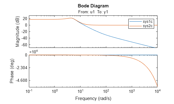
As the plot shows, the Bode responses of the two models do not match when you convert them to continuous time. When there is no feedthrough, as with sys1c, there must be some lag. When there is feedthrough, as with sys2c, there can be no lag. Continuous-time feedthrough maps to discrete-time feedthrough. Continuous-time lag maps to discrete-time delays.

Estimate a two-input, one-output discrete-time transfer function with a delay of two samples on the first input and zero samples on the second input. Both inputs have no feedthrough.

Load the data and split the data into estimation and validation data sets.

load iddata7 z7
ze = z7(1:300);
zv = z7(200:400);

Estimate a two-input, one-output transfer function with two poles and one zero for each input-to-output transfer function.

Lag = [2;0];
Ft = [false,false];
model = tfest(ze,2,1,'Ts',z7.Ts,'Feedthrough',Ft,'InputDelay',Lag);

The Feedthrough value you choose dictates whether the leading numerator coefficient is zero (no feedthrough) or not (nonzero feedthrough). Delays are generally expressed separately using the InputDelay or IODelay property. This example uses InputDelay only to express the delays.

Validate the estimated model. Exclude the data outliers for validation.

I = 1:201; 
I(114:118) = [];
opt = compareOptions('Samples',I);
compare(zv,model,opt)

Figure contains an axes object. The axes object with ylabel y1 contains 2 objects of type line. These objects represent Validation data (y1), model: 81.01%.

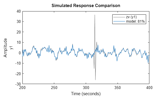
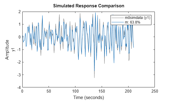
Identify a 15th order transfer function model by using regularized impulse response estimation.

Load the data.

load regularizationExampleData m0simdata;

Obtain a regularized impulse response (FIR) model.

opt = impulseestOptions('RegularizationKernel','DC');
m0 = impulseest(m0simdata,70,opt);

Convert the model into a transfer function model after reducing the order to 15.

m = idtf(balred(idss(m0),15));

Compare the model output with the data.

compare(m0simdata,m);

Figure contains an axes object. The axes object with ylabel y1 contains 2 objects of type line. These objects represent Validation data (y1), m: 63.82%.

Create an option set for tfest that specifies the initialization and search methods. Also set the display option, which specifies that the loss-function values for each iteration be shown.

opt = tfestOptions('InitializeMethod','n4sid','Display','on','SearchMethod','lsqnonlin');

Load time-domain system response data z2 and use it to estimate a transfer function with two poles and one zero. Specify opt for the estimation options.

load iddata2 z2;
np = 2;
nz = 1;
iodelay = 0.2;
sys = tfest(z2,np,nz,iodelay,opt);

sys is an idtf model containing the estimated transfer function.

Load the time-domain system response data z2, and use it to estimate a two-pole, one-zero transfer function. Specify an input delay.

load iddata2 z2;
np = 2;
nz = 1;
input_delay = 0.2;
sys = tfest(z2,np,nz,'InputDelay',input_delay);

sys is an idtf model containing the estimated transfer function with an input delay of 0.2 seconds.

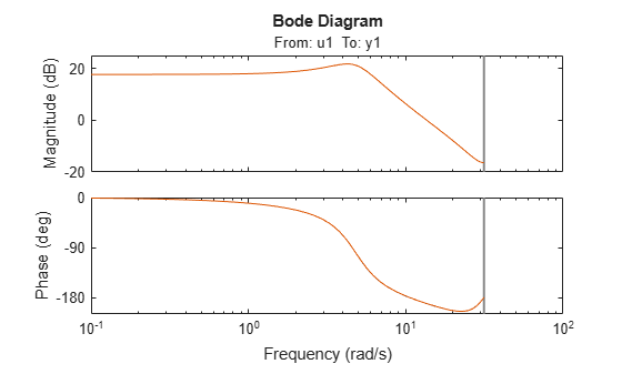
Use bode to obtain the magnitude and phase response for the following system:

H(s)=s+0.2s3+2s2+s+1

Use 100 frequency points, ranging from 0.1 rad/s to 10 rad/s, to obtain the frequency-response data. Use frd to create a frequency-response data object.

freq = logspace(-1,1,100);
[mag,phase] = bode(tf([1 0.2],[1 2 1 1]),freq);
data = frd(mag.*exp(1j*phase*pi/180),freq);

Estimate a three-pole, one-zero transfer function using data.

np = 3;
nz = 1;
sys = tfest(data,np,nz);

sys is an idtf model containing the estimated transfer function.

Load the time-domain system response data co2data, which contains the data from two experiments, each with two inputs and one output. Convert the data from the first experiment into an iddata object data with a sample time of 0.5 seconds.

load co2data;
Ts = 0.5;
data = iddata(Output_exp1,Input_exp1,Ts);

Specify estimation options for the search method and the input and output offsets. Also specify the maximum number of search iterations.

opt = tfestOptions('SearchMethod','gna');
opt.InputOffset = [170;50];
opt.OutputOffset = mean(data.y(1:75));
opt.SearchOptions.MaxIterations = 50;

Estimate a transfer function using the measured data and the estimation option set opt. Specify the transport delays from the inputs to the output.

np = 3;
nz = 1;
iodelay = [2 5];
sys = tfest(data,np,nz,iodelay,opt);

iodelay specifies the input-to-output delay from the first and second inputs to the output as 2 seconds and 5 seconds, respectively.

sys is an idtf model containing the estimated transfer function.

Load time-domain system response data and use it to estimate a transfer function for the system. Specify the known and unknown transport delays.

load co2data;
Ts = 0.5;
data = iddata(Output_exp1,Input_exp1,Ts);

data is an iddata object with two input channels and one output channels, and which has a sample rate of 0.5 seconds.

Create an option set opt. Specify estimation options for the search method and the input and output offsets. Also specify the maximum number of search iterations.

opt = tfestOptions('Display','on','SearchMethod','gna');
opt.InputOffset = [170; 50];
opt.OutputOffset = mean(data.y(1:75));
opt.SearchOptions.MaxIterations = 50;

Specify the unknown and known transport delays in iodelay, using 2 for a known delay of 2 seconds and nan for the unknown delay. Estimate the transfer function using iodelay and opt.

np = 3;
nz = 1;
iodelay = [2 nan];
sys = tfest(data,np,nz,iodelay,opt);

sys is an idtf model containing the estimated transfer function.

Create a transfer function model with the expected numerator and denominator structure and delay constraints.

In this example, the experiment data consists of two inputs and one output. Both transport delays are unknown and have an identical upper bound. Additionally, the transfer functions from both inputs to the output are identical in structure.

init_sys = idtf(NaN(1,2),[1,NaN(1,3)],'IODelay',NaN);
init_sys.Structure(1).IODelay.Free = true;
init_sys.Structure(1).IODelay.Maximum = 7;

init_sys is an idtf model describing the structure of the transfer function from one input to the output. The transfer function consists of one zero, three poles, and a transport delay. The use of NaN indicates unknown coefficients.

init_sys.Structure(1).IODelay.Free = true indicates that the transport delay is not fixed.

init_sys.Structure(1).IODelay.Maximum = 7 sets the upper bound for the transport delay to 7 seconds.

Specify the transfer function from both inputs to the output.

init_sys = [init_sys,init_sys];

Load time-domain system response data and use it to estimate a transfer function. Specify options in the tfestOptions option set opt.

load co2data;
Ts = 0.5; 
data = iddata(Output_exp1,Input_exp1,Ts);
opt = tfestOptions('Display','on','SearchMethod','gna');
opt.InputOffset = [170;50];
opt.OutputOffset = mean(data.y(1:75));
opt.SearchOptions.MaxIterations = 50;
sys = tfest(data,init_sys,opt);

sys is an idtf model containing the estimated transfer function.

Analyze the estimation result by comparison. Create a compareOptions option set opt2 and specify input and output offsets, and then use compare.

opt2 = compareOptions;
opt2.InputOffset = opt.InputOffset;
opt2.OutputOffset = opt.OutputOffset;
compare(data,sys,opt2)

Figure contains an axes object. The axes object with ylabel y1 contains 2 objects of type line. These objects represent Validation data (y1), sys: 66.19%.

Estimate a multiple-input, single-output transfer function containing different numbers of poles for input-output pairs for given data.

Obtain frequency-response data.

For example, use frd to create a frequency-response data model for the following system:

G=[e-4ss+2s3+2s2+4s+5e-0.6s5s4+2s3+s2+s]

Use 100 frequency points, ranging from 0.01 rad/s to 100 rad/s, to obtain the frequency-response data.

G = tf({[1 2],[5]},{[1 2 4 5],[1 2 1 1 0]},0,'IODelay',[4 0.6]);
data = frd(G,logspace(-2,2,100));

data is an frd object containing the continuous-time frequency response for G.

Estimate a transfer function for data.

 np = [3 4];
 nz = [1 0];
 iodelay = [4 0.6];
 sys = tfest(data,np,nz,iodelay);

np specifies the number of poles in the estimated transfer function. The first element of np indicates that the transfer function from the first input to the output contains three poles. Similarly, the second element of np indicates that the transfer function from the second input to the output contains four poles.

nz specifies the number of zeros in the estimated transfer function. The first element of nz indicates that the transfer function from the first input to the output contains one zero. Similarly, the second element of np indicates that the transfer function from the second input to the output does not contain any zeros.

iodelay specifies the transport delay from the first input to the output as 4 seconds. The transport delay from the second input to the output is specified as 0.6 seconds.

sys is an idtf model containing the estimated transfer function.

Estimate a transfer function describing an unstable system using frequency-response data.

Use idtf to construct a transfer function model G of the following system:

G=[s+2s3+2s2+4s+55s4+2s3+s2+s+1]

G = idtf({[1 2], 5},{[1 2 4 5],[1 2 1 1 1]});

Use idfrd to obtain a frequency-response data model data for G. Specify 100 frequency points ranging from 0.01 rad/s to 100 rad/s.

data = idfrd(G,logspace(-2,2,100));

data is an idfrd object.

Estimate a transfer function for data.

np = [3 4];
nz = [1 0];
sys = tfest(data,np,nz);

np specifies the number of poles in the estimated transfer function. The first element of np indicates that the transfer function from the first input to the output contains three poles. Similarly, the second element of np indicates that the transfer function from the second input to the output contains four poles.

nz specifies the number of zeros in the estimated transfer function. The first element of nz indicates that the transfer function from the first input to the output contains one zero. Similarly, the second element of nz indicates that the transfer function from the second input to the output does not contain any zeros.

sys is an idtf model containing the estimated transfer function.

pole(sys)
ans = 7×1 complex

  -1.5260 + 0.0000i
  -0.2370 + 1.7946i
  -0.2370 - 1.7946i
  -1.4656 + 0.0000i
  -1.0000 + 0.0000i
   0.2328 + 0.7926i
   0.2328 - 0.7926i

sys is an unstable system, as the pole display indicates.

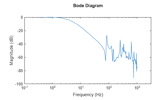
Load the high-density frequency-response measurement data. The data corresponds to an unstable process maintained at equilibrium using feedback control.

load HighModalDensityData FRF f

Package the data as an idfrd object for identification and find the Bode magnitude response.

G = idfrd(permute(FRF,[2 3 1]),f,0,'FrequencyUnit','Hz');
bodemag(G)

Figure contains an axes object. The axes object with ylabel Magnitude (dB) contains an object of type line. This object represents G.

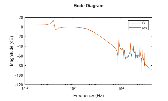
Estimate a transfer function with 32 poles and 32 zeros, and compare the Bode magnitude response.

sys = tfest(G,32,32);
bodemag(G, sys)
xlim([0.01,2e3])
legend

Figure contains an axes object. The axes object with ylabel Magnitude (dB) contains 2 objects of type line. These objects represent G, sys.

Load and plot the data.

load iddata1ic z1i
plot(z1i)

Figure contains 2 axes objects. Axes object 1 with title y1 contains an object of type line. This object represents z1i. Axes object 2 with title u1 contains an object of type line. This object represents z1i.

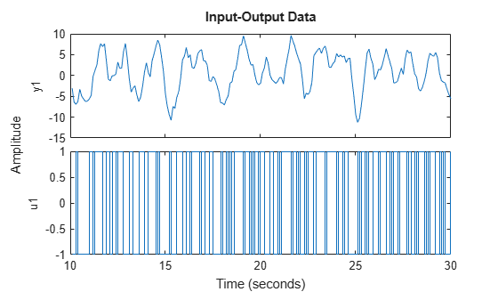
Examine the initial value of the output data y(1).

ystart = z1i.y(1)
ystart = -3.0491

The measured output does not start at 0.

Estimate a second-order transfer function sys and return the estimated initial condition ic.

[sys,ic] = tfest(z1i,2,1);
ic
ic = 
  initialCondition with properties:

     A: [2x2 double]
    X0: [2x1 double]
     C: [0.2957 5.2441]
    Ts: 0

ic is an initialCondition object that encapsulates the free response of sys, in state-space form, to the initial state vector in X0.

Simulate sys using the estimation data but without incorporating the initial conditions. Plot the simulated output with the measured output.

y_no_ic = sim(sys,z1i);
plot(y_no_ic,z1i)
legend('Model Response','Output Data')

Figure contains 2 axes objects. Axes object 1 with title y1 contains 2 objects of type line. These objects represent Model Response, Output Data. Axes object 2 with title u1 contains an object of type line. This object represents Output Data.

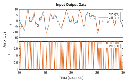
The measured and simulated outputs do not agree at the beginning of the simulation.

Incorporate the initial condition into the simOptions option set.

opt = simOptions('InitialCondition',ic);
y_ic = sim(sys,z1i,opt);
plot(y_ic,z1i)
legend('Model Response','Output Data')

Figure contains 2 axes objects. Axes object 1 with title y1 contains 2 objects of type line. These objects represent Model Response, Output Data. Axes object 2 with title u1 contains an object of type line. This object represents Output Data.

The simulation combines the model response to the input signal with the free response to the initial condition. The measured and simulated outputs now have better agreement at the beginning of the simulation. This initial condition is valid only for the estimation data z1i.

Input Arguments

collapse all

Estimation data, specified as a uniformly sampled timetable that contains both input and output signal variables or, for multiexperiment data, a cell array of timetables.

Use Entire Timetable

If you want to use all the input and output variables in tt, and the variables are organized so that the set of input variables is followed by the set of output variables, then:

  • For SISO systems, specify tt as an Ns-by-2 timetable, where Ns is the number of samples and the two timetable variables represent the measured input signal and output signal respectively.

  • For MIMO systems, specify tt as an Ns-by-(Nu+Ny) timetable, where Nu is the number of inputs and Ny is the number of outputs. The first Nu variables must contain the input signals and the remaining Ny variables must contain the output signals.

    When you are estimating state space or transfer function models, you must also explicitly specify the input and output channels, as the following section describes.

  • For multiexperiment data, specify data as an Ne-by-1 cell array of timetables, where Ne is the number of experiments. The sample times of all the experiments must match.

Use Selected Variables from Timetable

If you want to use a subset of variables from the timetable, or if the input and output variables are intermixed, use the 'InputName' and 'OutputName' name-value arguments to specify which variables to use.

For example, suppose that tt contains six variables: "u1", "u2", "u3", and "y1", "y2", "y3". For estimation, you want to use the variables "u1" and "u2" as the inputs and the variables "y1" and "y3" as the outputs. Use the following command to perform the estimation:

sys = tfest(tt,__,'InputName',["u1" "u2"],'OutputName',["y1" "y3"])

For more information about working with estimation data types, see Data Domains and Data Types in System Identification Toolbox.

Estimation data, specified for SISO systems as a pair of Ns-by-1 real-valued matrices that contain uniformly sampled input and output time-domain signal values. Here, Ns is the number of samples.

For MIMO systems, specify u,y as an input/output matrix pair with the following dimensions:

  • uNs-by-Nu, where Nu is the number of inputs.

  • yNs-by-Ny, where Ny is the number of outputs.

For multiexperiment data, specify u,y as a pair of 1-by-Ne cell arrays, where Ne is the number of experiments. The sample times of all the experiments must match.

Limitations

  • Matrix-based data does not support estimation from frequency-domain data. You must use a data object such as an iddata object or idfrd object (see data).

  • Using matrices for estimation data is not recommended for continuous-time estimation since the data does not provide the sample time. The software assumes that the data is sampled at 1 Hz. For continuous-time estimation, it is recommended that you convert the input and output matrix pair into a single timetable. For example, to convert the single-column matrices um and ym to a timetable tt with a sample time of 0.5 minutes, use the following command.

    tt = timetable(um,ym,'rowtimes',minutes(0.5*(1:size(u,1))))
    For a more detailed example of converting matrix-based SISO data to a timetable, see Convert SISO Matrix Data to Timetable. For an example of converting a MIMO matrix pair to a timetable, see Convert MIMO Matrix Data to Timetable for Continuous-Time Model Estimation.

    For more information about working with estimation data types, see Data Domains and Data Types in System Identification Toolbox.

Estimation data object, specified as an iddata object, an frd object, or an idfrd object that contains uniformly sampled input and output values. By default, the software sets the sample time of the model to the sample time of the estimation data.

For multiexperiment data, the sample times and intersample behavior of all the experiments must match.

For time-domain estimation, data must be an iddata object containing the input and output signal values.

For frequency-domain estimation, data can be one of the following:

  • Recorded frequency response data (frd (Control System Toolbox) or idfrd)

  • iddata object with properties specified as follows:

    • InputData — Fourier transform of the input signal

    • OutputData — Fourier transform of the output signal

    • Domain'Frequency'

Limitations

You cannot estimate continuous-time models using discrete-time frequency-domain data.

Number of poles in the estimated transfer function, specified as a nonnegative integer or a matrix.

For systems that have multiple inputs and/or multiple outputs, you can apply either a global value or individual values of np to the input/output pairs, as follows:

  • Same number of poles for every pair — Specify np as a scalar.

  • Individual number of poles for each pair — Specify np as an Ny-by-Nu matrix. Ny is the number of outputs and Nu is the number of inputs.

For an example, see Estimate Transfer Function Model by Specifying Number of Poles.

Number of zeros in the estimated transfer function, specified as a nonnegative integer or a matrix.

For systems that have multiple inputs, multiple outputs, or both, you can apply either a global value or individual values of nz to the input/output pairs, as follows:

  • Same number of poles for every pair — Specify nz as a scalar.

  • Individual number of poles for each pair — Specify nz as an Ny-by-Nu matrix. Ny is the number of outputs and Nu is the number of inputs.

For a continuous-time model estimated using discrete-time data, set nz <= np.

For discrete-time model estimation, specify nz as the number of zeros of the numerator polynomial of the transfer function. For example, tfest(tt,2,1,'Ts',data.Ts) estimates a transfer function of the form b1z1/(1+a1z1+b2z2), while tfest(tt,2,2,'Ts',data.Ts) estimates (b1z1+b2z2)/(1+a1z1+b2z2). Here, z-1 is the Z-transform lag variable. For more information about discrete-time transfer functions, see Discrete-Time Representation. For an example, see Estimate Discrete-Time Transfer Function.

Transport delay, specified as a nonnegative integer, a NaN scalar, or a matrix.

For continuous-time systems, specify transport delays in the time unit stored in the TimeUnit property of data. For discrete-time systems, specify transport delays as integers denoting delays of a multiple of the sample time Ts.

For a MIMO system with Ny outputs and Nu inputs, set iodelay to an Ny-by-Nu array. Each entry of this array is a numerical value that represents the transport delay for the corresponding input/output pair. You can also set iodelay to a scalar value to apply the same delay to all input/output pairs.

The specified values are treated as fixed delays. To denote unknown transport delays, specify NaN in the iodelay matrix.

Use [] or 0 to indicate no transport delay.

For an example, see Estimate Transfer Function Containing Known Transport Delay.

Estimation options, specified as a tfestOptions option set. Options specified by opt include:

  • Estimation objective

  • Handling of initial conditions

  • Numerical search method to be used in estimation

  • Intersample behavior

For an example, see Estimate Transfer Function Using Estimation Option Set.

Linear system that configures the initial parameterization of sys, specified as an idtf model, a linear model , or a structure. You obtain init_sys either by performing an estimation using measured data or by direct construction.

If init_sys is an idtf model, tfest uses the parameter values of init_sys as the initial guess for estimating sys.

Use the Structure property of init_sys to configure initial parameter values and constraints for the numerator, denominator, and transport lag. For instance:

  • To specify an initial guess for the A matrix of init_sys, set init_sys.Structure.Numerator.Value to the initial guess.

  • To specify constraints for the B matrix of init_sys:

    • Set init_sys.Structure.Numerator.Minimum to the minimum numerator coefficient values.

    • Set init_sys.Structure.Numerator.Maximum to the maximum numerator coefficient values.

    • Set init_sys.Structure.Numerator.Free to indicate which numerator coefficients are free for estimation.

    For an example, see Estimate Transfer Function with Unknown, Constrained Transport Delays.

If init_sys is not an idtf model, the software first converts init_sys to a transfer function. tfest uses the parameters of the resulting model as the initial guess for estimation.

If you do not specify opt, and init_sys was obtained by estimation rather than construction, then the software uses estimation options from init_sys.Report.OptionsUsed.

Name-Value Arguments

Specify optional pairs of arguments as Name1=Value1,...,NameN=ValueN, where Name is the argument name and Value is the corresponding value. Name-value arguments must appear after other arguments, but the order of the pairs does not matter.

Before R2021a, use commas to separate each name and value, and enclose Name in quotes.

Example: sys = tfest(data,np,nz,'Ts',0.1)

Input channel names, specified as a string, character vector, string array, or cell array of character vectors.

If you are using a timetable for the data source, the names in InputName must be a subset of the timetable variables.

Example: sys = tfest(tt,__,'InputName',["u1" "u2"]) selects the variables u1 and u2 as the input channels from the timetable tt to use for the estimation.

Output channel names, specified as a string, character vector, string array, or cell array of character vectors.

If you are using a timetable for the data source, the names in OutputName must be a subset of the timetable variables.

Example: sys = tfest(tt,__,'OutputName',["y1" "y3"]) selects the variables y1 and y3 as the output channels from the timetable tt to use for the estimation.

Sample time of the estimated model, specified as either 0 or a positive scalar.

  • For continuous-time models, specify 'Ts' as 0.

  • For discrete-time models, specify 'Ts' as the data sample time in units defined by the following:

    • For timetable-based data — The timetable Time column

    • For matrix-based data — Seconds

    • For data objects, such as iddata objects — The data.TimeUnit property

    In the discrete case, np and nz refer to the number of roots of z-1 for the numerator and denominator polynomials.

    To obtain the data sample time for a timetable tt, use the timetable property tt.Properties.Timestep.

For an example, see Estimate Discrete-Time Transfer Function.

Input delay for each input channel, specified as a scalar or a numeric vector.

  • For continuous-time models, specify 'InputDelay' in the time units stored in the TimeUnit property.

  • For discrete-time models, specify 'InputDelay' in integer multiples of the sample time Ts. For example, setting 'InputDelay' to 3 specifies a delay of three sampling periods.

For a system with Nu inputs, set InputDelay to an Nu-by-1 vector. Each entry of this vector is a numerical value that represents the input delay for the corresponding input channel.

To apply the same delay to all channels, specify InputDelay as a scalar.

For an example, see Specify Model Properties of Estimated Transfer Function.

Feedthrough for discrete-time transfer functions, specified as a logical scalar or an Ny-by-Nu logical matrix. Ny is the number of outputs and Nu is the number of inputs. To use the same feedthrough for all input/output channels, specify Feedthrough as a scalar.

Consider a discrete-time model with two poles and three zeros:

H(z1)=b0+b1z1+b2z2+b3z31+a1z1+a2z2

When the model has direct feedthrough, b0 is a free parameter whose value is estimated along with the rest of the model parameters b1, b2, b3, a1, and a2. When the model has no feedthrough, b0 is fixed to zero. For an example, see Estimate Discrete-Time Transfer Function with Feedthrough.

Output Arguments

collapse all

Identified transfer function, returned as an idtf model. This model is created using the specified model orders, delays, and estimation options.

Information about the estimation results and options used is stored in the Report property of the model. Report has the following fields.

Report FieldDescription
Status

Summary of the model status, which indicates whether the model was created by construction or obtained by estimation.

Method

Estimation command used.

InitializeMethod

Algorithm used to initialize the numerator and denominator for estimation of continuous-time transfer functions using time-domain data, returned as one of the following values:

  • 'iv' — Instrument Variable approach

  • 'svf' — State Variable Filters approach

  • 'gpmf' — Generalized Poisson Moment Functions approach

  • 'n4sid' — Subspace state-space estimation approach

This field is especially useful to view the algorithm used when the InitializeMethod option in the estimation option set is 'all'.

N4Weight

Weighting matrices used in the singular-value decomposition step when InitializeMethod is 'n4sid', returned as one of the following values:

  • 'MOESP' — Use the MOESP algorithm by Verhaegen.

  • 'CVA' — Use the canonical variate algorithm (CVA) by Larimore.

  • 'SSARX' — Use a subspace identification method that uses an ARX estimation-based algorithm to compute the weighting.

This field is especially useful to view the weighting matrices used when the N4Weight option in the estimation option set is 'auto'.

N4Horizon

Forward and backward prediction horizons used when InitializeMethod is 'n4sid', returned as a row vector with three elements — [r sy su], where r is the maximum forward prediction horizon, sy is the number of past outputs, and su is the number of past inputs that are used for the predictions.

InitialCondition

Handling of initial conditions during model estimation, returned as one of the following values:

  • 'zero' — The initial conditions were set to zero.

  • 'estimate' — The initial conditions were treated as independent estimation parameters.

  • 'backcast' — The initial conditions were estimated using the best least squares fit.

This field is especially useful to view how the initial conditions were handled when the InitialCondition option in the estimation option set is 'auto'.

Fit

Quantitative assessment of the estimation, returned as a structure. See Loss Function and Model Quality Metrics for more information on these quality metrics. The structure has the following fields:

FieldDescription
FitPercent

Normalized root mean squared error (NRMSE) measure of how well the response of the model fits the estimation data, expressed as the percentage fitpercent = 100(1-NRMSE).

LossFcn

Value of the loss function when the estimation completes.

MSE

Mean squared error (MSE) measure of how well the response of the model fits the estimation data.

FPE

Final prediction error for the model.

AIC

Raw Akaike Information Criteria (AIC) measure of model quality.

AICc

Small-sample-size corrected AIC.

nAIC

Normalized AIC.

BIC

Bayesian Information Criteria (BIC).

Parameters

Estimated values of model parameters.

OptionsUsed

Option set used for estimation. If no custom options were configured, this is a set of default options. See polyestOptions for more information.

RandState

State of the random number stream at the start of estimation. Empty, [], if randomization was not used during estimation. For more information, see rng.

DataUsed

Attributes of the data used for estimation, returned as a structure with the following fields.

FieldDescription
Name

Name of the data set.

Type

Data type.

Length

Number of data samples.

Ts

Sample time.

InterSample

Input intersample behavior, returned as one of the following values:

  • 'zoh' — Zero-order hold maintains a piecewise-constant input signal between samples.

  • 'foh' — First-order hold maintains a piecewise-linear input signal between samples.

  • 'bl' — Band-limited behavior specifies that the continuous-time input signal has zero power above the Nyquist frequency.

InputOffset

Offset removed from time-domain input data during estimation. For nonlinear models, it is [].

OutputOffset

Offset removed from time-domain output data during estimation. For nonlinear models, it is [].

Termination

Termination conditions for the iterative search used for prediction error minimization, returned as a structure with the following fields:

FieldDescription
WhyStop

Reason for terminating the numerical search.

Iterations

Number of search iterations performed by the estimation algorithm.

FirstOrderOptimality

-norm of the gradient search vector when the search algorithm terminates.

FcnCount

Number of times the objective function was called.

UpdateNorm

Norm of the gradient search vector in the last iteration. Omitted when the search method is 'lsqnonlin' or 'fmincon'.

LastImprovement

Criterion improvement in the last iteration, expressed as a percentage. Omitted when the search method is 'lsqnonlin' or 'fmincon'.

Algorithm

Algorithm used by 'lsqnonlin' or 'fmincon' search method. Omitted when other search methods are used.

For estimation methods that do not require numerical search optimization, the Termination field is omitted.

For more information on using Report, see Estimation Report.

Estimated initial conditions, returned as an initialCondition object or an object array of initialCondition values.

  • For a single-experiment data set, ic represents, in state-space form, the free response of the transfer function model (A and C matrices) to the estimated initial states (x0).

  • For a multiple-experiment data set with Ne experiments, ic is an object array of length Ne that contains one set of initialCondition values for each experiment.

If tfest returns ic values of 0 and you know that you have non-zero initial conditions, set the 'InitialCondition' option in tfestOptions to 'estimate' and pass the updated option set to tfest. For example:

opt = tfestOptions('InitialCondition','estimate')
[sys,ic] = tfest(data,np,nz,opt)
The default 'auto' setting of 'InitialCondition' uses the 'zero' method when the initial conditions have a negligible effect on the overall estimation-error minimization process. Specifying 'estimate' ensures that the software estimates values for ic.

For more information, see initialCondition. For an example of using this argument, see Obtain and Apply Estimated Initial Conditions.

Algorithms

collapse all

The details of the estimation algorithms used by tfest vary depending on various factors, including the sampling of the estimated model and the estimation data.

Continuous-Time Transfer Function Estimation Using Time-Domain Data

Parameter Initialization

The estimation algorithm initializes the estimable parameters using the method specified by the InitializeMethod estimation option. The default method is the Instrument Variable (IV) method.

The State-Variable Filters (SVF) approach and the Generalized Poisson Moment Functions (GPMF) approach to continuous-time parameter estimation use prefiltered data [1] [2]. The constant 1λ in [1] and [2] corresponds to the initialization option (InitializeOptions) field FilterTimeConstant. IV is the simplified refined IV method and is called SRIVC in [3]. This method has a prefilter that is the denominator of the current model, initialized with SVF. This prefilter is iterated up to MaxIterations times, until the model change is less than Tolerance. MaxIterations and Tolerance are options that you can specify using the InitializeOptions structure. The 'n4sid' initialization option estimates a discrete-time model, using the N4SID estimation algorithm, that it transforms to continuous-time using d2c.

Use tfestOptions to create the option set used to estimate a transfer function.

Parameter Update

The initialized parameters are updated using a nonlinear least-squares search method, specified by the SearchMethod estimation option. The objective of the search method is to minimize the weighted prediction error norm.

Discrete-Time Transfer Function Estimation Using Time-Domain Data

For discrete-time data, tfest uses the same algorithm as oe to determine the numerator and denominator polynomial coefficients. In this algorithm, the initialization is performed using arx, followed by nonlinear least-squares search-based updates to minimize a weighted prediction error norm.

Continuous-Time Transfer Function Estimation Using Continuous-Time Frequency-Domain Data

The estimation algorithm performs the following tasks:

  1. Perform a bilinear mapping to transform the domain (frequency grid) of the transfer function. For continuous-time models, the imaginary axis is transformed to the unit disk. For discrete-time models, the original domain unit disk is transformed to another unit disk.

  2. Perform S-K iterations [4] to solve a nonlinear least-squares problem — Consider a multi-input single-output system. The nonlinear least-squares problem is to minimize the following loss function:

    minimizeD,Nik=1nf|W(ωk)(y(ωk)i=1nuNi(ωk)D(ωk)ui(ωk))|2

    Here, W is a frequency-dependent weight that you specify. D is the denominator of the transfer function model that is to be estimated, and Ni is the numerator corresponding to the ith input. y and u are the measured output and input data, respectively. nf and nu are the number of frequencies and inputs, and w is the frequency. Rearranging the terms gives

    minimizeD,Nik=1nf|W(ωk)D(ωk)(D(ωk)y(ωk)i=1nuNi(ωk)ui(ωk))|2

    To perform the S-K iterations, the algorithm iteratively solves

    minimizeDm,Ni,mk=1nf|W(ωk)Dm1(ωk)(Dm(ωk)y(ωk)i=1nuNi,m(ωk)ui(ωk))|2

    Here, m is the current iteration, and Dm-1(ω) is the denominator response identified at the previous iteration. Now each step of the iteration is a linear least-squares problem, where the identified parameters capture the responses Dm(ω) and Ni,m(ω) for i = 1,2,...nu. The iteration is initialized by choosing D0(ω) = 1.

    • The first iteration of the algorithm identifies D1(ω). The D1(ω) and Ni,1(ω) polynomials are expressed in monomial basis.

    • The second and following iterations express the polynomials Dm(ω) and Ni,m(ω) in terms of orthogonal rational basis functions on the unit disk. These basis functions have the form

      Bj,m(ω)=(1|λj,m1|2qλj,m1)r=0j11(λj,m1)*q(ω)q(ω)λr,m1

      Here, λj,m-1 is the jth pole that is identified at the previous step m-1 of the iteration. λj,m-1* is the complex conjugate of λj,m-1, and q is the frequency-domain variable on the unit disk.

    • The algorithm runs for a maximum of 20 iterations. The iterations are terminated early if the relative change in the value of the loss function is less than 0.001 in the last three iterations.

    If you specify bounds on transfer function coefficients, these bounds correspond to affine constraints on the identified parameters. If you have only equality constraints (fixed transfer function coefficients), the corresponding equality constrained least-squares problem is solved algebraically. To do so, the software computes an orthogonal basis for the null space of the equality constraint matrix, and then solves the least-squares problem within this null space. If you have upper or lower bounds on transfer function coefficients, the corresponding inequality constrained least-squares problem is solved using interior-point methods.

  3. Perform linear refinements — The S-K iterations, even when they converge, do not always yield a locally optimal solution. To find a critical point of the optimization problem that can yield a locally optimal solution, a second set of iterations are performed. The critical points are solutions to a set of nonlinear equations. The algorithm searches for a critical point by successively constructing a linear approximation to the nonlinear equations and solving the resulting linear equations in the least-squares sense. The equations follow.

    • Equation for the jth denominator parameter:

      0=2k=1nfRe{|W(ωk)|2Bj*(ωk)i=1nuNi,m1*(ωk)ui*(ωk)Dm1*(ωk)|Dm1(ωk)|2(Dm(ωk)y(ωk)i=1nuNi,m(ωk)ui(ωk))}

    • Equation for the jth numerator parameter that corresponds to input l:

      0=2k=1nfRe{|W(ωk)|2Bj*(ωk)ul*(ωk)|Dm1(ωk)|2(Dm(ωk)y(ωk)i=1nuNi,m(ωk)ui(ωk))}

    The first iteration is started with the best solution found for the numerators Ni and denominator D parameters during S-K iterations. Unlike S-K iterations, the basis functions Bj(ω) are not changed at each iteration; the iterations are performed with the basis functions that yielded the best solution in the S-K iterations. As before, the algorithm runs for a maximum of 20 iterations. The iterations are terminated early if the relative change in the value of the loss function is less than 0.001 in the last three iterations.

    If you specify bounds on transfer function coefficients, these bounds are incorporated into the necessary optimality conditions using generalized Lagrange multipliers. The resulting constrained linear least-squares problems are solved using the same methods explained in the S-K iterations step.

  4. Return the transfer function parameters corresponding to the optimal solution — Both the S-K and linear refinement iteration steps do not guarantee an improvement in the loss function value. The algorithm tracks the best parameter value observed during these steps, and returns these values.

  5. Invert the bilinear mapping performed in step 1.

  6. Perform an iterative refinement of the transfer function parameters using the nonlinear least-squares search method specified in the SearchMethod estimation option. This step is implemented in the following situations:

    • When you specify the EnforceStability estimation option as true (stability is requested), and the result of step 5 of this algorithm is an unstable model. The unstable poles are reflected inside the stability boundary and the resulting parameters are iteratively refined. For information about estimation options, see tfestOptions.

    • When you add a regularization penalty to the loss function using the Regularization estimation option. For an example about regularization, see Regularized Identification of Dynamic Systems.

    • You estimate a continuous-time model using discrete-time data (see Discrete-Time Transfer Function Estimation Using Discrete-Time Frequency-Domain Data).

    • You use frequency domain input/output data to identify a multi-input model.

If you are using the estimation algorithm from R2016a or earlier (see tfest Estimation Algorithm Update) for estimating a continuous-time model using continuous-time frequency-domain data, then for continuous-time data and fixed delays, the Output-Error algorithm is used for model estimation. For continuous-time data and free delays, the state-space estimation algorithm is used. In this algorithm, the model coefficients are initialized using the N4SID estimation method. This initialization is followed by nonlinear least-squares search-based updates to minimize a weighted prediction error norm.

Discrete-Time Transfer Function Estimation Using Discrete-Time Frequency-Domain Data

The estimation algorithm is the same as for continuous-time transfer function estimation using continuous-time frequency-domain data, except discrete-time data is used.

If you are using the estimation algorithm from R2016a or earlier (see tfest Estimation Algorithm Update), the algorithm is the same as the algorithm for discrete-time transfer function estimation using time-domain data.

Note

The software does not support estimation of a discrete-time transfer function using continuous-time frequency-domain data.

Continuous-Time Transfer Function Estimation Using Discrete-Time Frequency-Domain Data

The tfest command first estimates a discrete-time model from the discrete-time data. The estimated model is then converted to a continuous-time model using the d2c command. The frequency response of the resulting continuous-time model is then computed over the frequency grid of the estimation data. A continuous-time model of the desired (user-specified) structure is then fit to this frequency response. The estimation algorithm for using the frequency-response data to obtain the continuous-time model is the same as the algorithm for continuous-time transfer function estimation using continuous-time data.

If you are using the estimation algorithm from R2016a or earlier (see tfest Estimation Algorithm Update), the state-space estimation algorithm is used for estimating continuous-time models from discrete-time data. In this algorithm, the model coefficients are initialized using the N4SID estimation method. This initialization is followed by nonlinear least-squares search-based updates to minimize a weighted prediction error norm.

Delay Estimation

  • When delay values are specified as NaN, the software uses delayest to estimate them separately from the model numerator and denominator coefficients. tfest then treats these delay values as fixed during the iterative update of the rest of the model. Therefore, the delay values are not iteratively updated.

  • By default, for discrete-time data (Ts>0), delayest limits the search for delays to a range of 0–30 samples. For continuous-time models, this range translates to 0–30Ts time units. For continuous-time data (Ts = 0), delayest limits the search range to 0–10 time units. You can change these limits by first creating a template model init_sys using idtf and then, setting the values of init_sys.Structure.IODelay.Minimum and init_sys.Structure(i,j).IODelay.Maximum.

  • For an initial model, init_sys, with:

    • init_sys.Structure.IODelay.Value specified as finite values

    • init_sys.Structure.IODelay.Free specified as true

    the initial delay values are left unchanged.

Estimation of delays is often a difficult problem. A best practice is to assess the presence and the value of a delay. To do so, use physical insight of the process being modeled and functions such as arxstruc, delayest, and impulseest. For an example of determining input delay, see Model Structure Selection: Determining Model Order and Input Delay.

References

[1] Garnier, H., M. Mensler, and A. Richard. “Continuous-Time Model Identification from Sampled Data: Implementation Issues and Performance Evaluation.” International Journal of Control 76, no. 13 (January 2003): 1337–57. https://doi.org/10.1080/0020717031000149636.

[2] Ljung, Lennart. “Experiments with Identification of Continuous Time Models.” IFAC Proceedings Volumes 42, no. 10 (2009): 1175–80. https://doi.org/10.3182/20090706-3-FR-2004.00195.

[3] Young, Peter, and Anthony Jakeman. “Refined Instrumental Variable Methods of Recursive Time-Series Analysis Part III. Extensions.” International Journal of Control 31, no. 4 (April 1980): 741–64. https://doi.org/10.1080/00207178008961080.

[4] Drmač, Z., S. Gugercin, and C. Beattie. “Quadrature-Based Vector Fitting for Discretized H2 Approximation.” SIAM Journal on Scientific Computing 37, no. 2 (January 2015): A625–52. https://doi.org/10.1137/140961511.

[5] Ozdemir, Ahmet Arda, and Suat Gumussoy. “Transfer Function Estimation in System Identification Toolbox via Vector Fitting.” IFAC-PapersOnLine 50, no. 1 (July 2017): 6232–37. https://doi.org/10.1016/j.ifacol.2017.08.1026.

Version History

Introduced in R2012a

expand all