Main Content

idfrd

Frequency response data or model

Description

An idfrd object stores frequency response data over a range of frequency values. You can use an idfrd object in two ways. You can use the object as estimation data for estimating a time-domain or frequency-domain model, similarly to an iddata object. Or, you can use the object as a linear model, similarly to how you use an idss state-space model or any other identified linear model. Use the idfrd command to encapsulate frequency response data or to convert a linear time-domain or frequency-domain dynamic model into a frequency response model.

Commands that accept iddata objects, such as the model estimation command ssest, generally also accept idfrd objects. However, an idfrd object can contain data from only one experiment. It does not have the multiexperiment capability that an iddata object has.

Commands that accept identified linear models, such as the analysis and validation commands compare, sim, and bode, generally also accept idfrd models.

For a model of the form

y(t)=G(q)u(t)+H(q)e(t)

the transfer function estimate is G(eiω) and the additive noise spectrum Φv at the output is

Φv(ω)=λT|H(eiωT)|2

Here, λ is the estimated variance of e(t) and T is the sample time.

For a continuous-time system, the noise spectrum is

Φv(ω)=λ|H(eiω)|2

An idfrd object stores G(eiω) and Φv.

Creation

You can obtain an idfrd model in one of three ways.

  • Create the model from frequency response data using the idfrd command. For example, create an idfrd model that encapsulates frequency response data taken at specific frequencies using the sample time Ts.

    sysfr = idfrd(ResponseData,Freq,Ts)
    For an example, see Create idfrd Object from Frequency Response Data.

  • Estimate the model using a frequency response estimation command such as spa, using time-domain, frequency-domain, or frequency response data.

    sysfr = spa(data)

    For more information about frequency response estimation commands, see spa, spafdr, and etfe.

  • Convert a linear model such as an idss model into an idfrd model by computing the frequency response of the model.

    sysfr = idfrd(sys)
    For an example of linear model conversion, see Convert Time-Domain Model to Frequency Response Model.

For information on functions you can use to extract information from or transform idfrd model objects, see Object Functions.

Description

Create Frequency Response Object

example

sysfr = idfrd(ResponseData,Frequency,Ts) creates a discrete-time idfrd object that stores the frequency response ResponseData of a linear system at frequency values Frequency. Ts is the sample time. For a continuous-time system, set Ts to 0.

sysfr = idfrd(___,Name,Value) sets additional properties using one or more name-value arguments. Specify the name-value arguments after the first three arguments. For instance, to specify the frequency units as MHz, use sysfr = idfrd(ResponseData,Frequency,Ts,'FrequencyUnits','MHz').

Convert Linear Identified Model to Frequency Response Model

example

sysfr = idfrd(sys) converts a System Identification Toolbox™ or Control System Toolbox™ linear model to frequency response data at default frequencies, including the output noise spectra and spectra covariance.

sysfr = idfrd(sys,Frequency) computes the frequency response at frequencies Frequency, where Frequency is expressed in radians/TimeUnit.

sysfr = idfrd(sys,Frequency,FrequencyUnits) interprets frequencies in the Frequency vector in the units specified by FrequencyUnit.

Input Arguments

expand all

Linear dynamic system model, specified as a System Identification Toolbox or Control System Toolbox linear model.

Properties

expand all

Frequency response data, specified as a 3-D array of complex numbers.

  • For SISO systems, ResponseData is a vector of frequency response values at the frequency points specified in the Frequency property.

  • For MIMO systems with Nu inputs and Ny outputs, ResponseData is an Ny-by-Nu-by-Nf array, where Nf is the number of frequency points.

    ResponseData(ky,ku,kf) represents the frequency response from the input ku to the output ky at the frequency Frequency(kf).

Frequency points corresponding to ResponseData, specified as a column vector that contains Nf points in the units specified by FrequencyUnit.

Units of the frequency vector in the Frequency property, specified as one of the following values:

  • 'rad/TimeUnit'

  • 'cycles/TimeUnit'

  • 'rad/s'

  • 'Hz'

  • 'kHz'

  • 'MHz'

  • 'GHz'

  • 'rpm'

The units 'rad/TimeUnit' and 'cycles/TimeUnit' are relative to the time units specified in the TimeUnit property.

Changing this property does not resample or convert the data. Modifying the property changes only the interpretation of the existing data. Use chgTimeUnit to convert the data to different frequency units.

Power spectra and cross spectra of the system output disturbances (noise), specified as a vector (single-output system) or a 3-D array of complex numbers (multiple-output system). For response data with Ny outputs and Nf frequency points, specify SpectrumData as an Ny-by-Ny-by-Nf array.

SpectrumData(ky1,ky2,kf) is the cross spectrum between the noise at output ky1 and the noise at output ky2 at the frequency Frequency(kf). The power spectrum is the subset of the cross spectrum where ky1 and ky2 are equal.

Covariance of SpectrumData, specified as a 5-D array with dimensions Ny-by-Nu-by-Nf-by-2-by-2, where Ny is the number of outputs, Nu is the number of inputs, and Nf is the number of frequency points.

CovarianceData(ky,ku,kf,:,:) is the 2-by-2 covariance matrix of SpectrumData(ky,ku,kf). The (1,1) element is the variance of the real part, the (2,2) element is the variance of the imaginary part, and the (1,2) and (2,1) elements are the covariance between the real and imaginary parts. squeeze(CovarianceData(ky,ku,kf,:,:)) thus gives the covariance matrix of the corresponding response.

If you obtain sysfr by converting a model sys, the value of CovarianceData depends on how you obtained sys.

  • If you obtained sys by identification, the software computes the estimated covariance for sysfr from the uncertainty information in sys. The software uses Gauss' approximation formula for this calculation for all model types, except grey-box models. For grey-box models (idgrey), the software applies numerical differentiation.

  • If you created sys by using commands such as idss, idtf, idproc, idgrey, or idpoly, then the software sets CovarianceData for sysfr to [].

Power spectra variance, specified as a vector (single-output system) or a 3-D array (multiple-output system). For response data with Ny outputs and Nf frequency points, specify NoiseCovariance as an Ny-by-Ny-by-Nf array. NoiseCovariance(ky1,ky2,kf) is the variance of the corresponding power spectrum.

To eliminate the influence of the noise component from the model, specify NoiseCovariance as 0. With zero covariance, the predicted output is the same as the simulated output.

Intersample behavior of the input signal for transformations between discrete time and continuous time, specified as a character vector or as an Nu-by-1 cell array of character vectors, where Nu is the number of input channels. This property is meaningful only when you are estimating continuous-time models (sample time Ts > 0) from discrete-time data.

For each input channel, the possible values of InterSample are:

  • 'zoh' — Zero-order hold maintains a piecewise-constant input signal between samples.

  • 'foh' — First-order hold maintains a piecewise-linear input signal between samples.

  • 'bl' — Band-limited behavior specifies that the continuous-time input signal has zero power above the Nyquist frequency (pi/sys.Ts rad/s). This behavior typically occurs when the input signal is measured experimentally using an antialiasing filter and a sampler. Ideally, treat the data as continuous-time. That is, if the signals used for the estimation of the frequency response were subject to anti-aliasing filters, set sys.Ts to zero.

If you obtain sysfr by conversion of a model sys, then InterSample is equal to the Intersample property of the iddata object that you used to estimate sys.

For more information on this property, see Effect of Input Intersample Behavior on Continuous-Time Models.

Transport delays, specified as a numeric array containing a separate transport delay for each input-output pair.

For continuous-time systems, transport delays are expressed in the time unit stored in the TimeUnit property. For discrete-time systems, transport delays are expressed as integers denoting delays of a multiple of the sample time Ts.

For a MIMO system with Ny outputs and Nu inputs, set IODelay as an Ny-by-Nu array. Each entry of this array is a numerical value representing the transport delay for the corresponding input-output pair. You can set IODelay to a scalar value to apply the same delay to all input-output pairs.

Input delay for each input channel, specified as a scalar value or numeric vector. For continuous-time systems, specify input delays in the time unit stored in the TimeUnit property. For discrete-time systems, specify input delays in integer multiples of the sample time Ts. For example, setting InputDelay to 3 specifies a delay of three sample times.

For a system with Nu inputs, set InputDelay to an Nu-by-1 vector. Each entry of this vector is a numerical value that represents the input delay for the corresponding input channel.

You can also set InputDelay to a scalar value to apply the same delay to all channels.

For identified systems such as idfrd, OutputDelay is fixed to zero.

Sample time, specified as one of the following.

  • Discrete-time model with a specified sampling time — a positive scalar representing the sampling period expressed in the unit specified by the TimeUnit property of the model

  • Continuous-time model — 0

  • Discrete-time model with an unspecified sample time — -1

Changing this property does not discretize or resample the model. Use c2d and d2c to convert between continuous- and discrete-time representations. Use d2d to change the sample time of a discrete-time system.

Units for the time variable, the sample time Ts, and any time delays in the model, specified as one of the following values.

  • 'nanoseconds'

  • 'microseconds'

  • 'milliseconds'

  • 'seconds'

  • 'minutes'

  • 'hours'

  • 'days'

  • 'weeks'

  • 'months'

  • 'years'

Changing this property does not resample or convert the data. Modifying the property changes only the interpretation of the existing data. Use chgTimeUnit (Control System Toolbox) to convert data to different time units

Input channel names, specified as a character vector or cell array.

  • Single-input model — Character vector. For example, 'controls'.

  • Multi-input model — Cell array of character vectors.

Alternatively, use automatic vector expansion to assign input names for multi-input models. For example, if sys is a two-input model, enter:

sys.InputName = 'controls';

The input names automatically expand to {'controls(1)';'controls(2)'}.

When you estimate a model using an iddata object data, the software automatically sets InputName to data.InputName.

You can use the shorthand notation u to refer to the InputName property. For example, sys.u is equivalent to sys.InputName.

You can use input channel names in several ways, including:

  • To identify channels on model display and plots

  • To extract subsystems of MIMO systems

  • To specify connection points when interconnecting models

Input channel units, specified as a character vector or cell array:

  • Single-input model — Character vector

  • Multi-input Model — Cell array of character vectors

Use InputUnit to keep track of input signal units. InputUnit has no effect on system behavior.

Input channel groups, specified as a structure. The InputGroup property lets you divide the input channels of MIMO systems into groups so that you can refer to each group by name. In the InputGroup structure, set field names to the group names, and field values to the input channels belonging to each group.

For example, create input groups named controls and noise that include input channels 1 and 2 and channels 3 and 5, respectively.

sys.InputGroup.controls = [1 2];
sys.InputGroup.noise = [3 5];

You can then extract the subsystem from the controls inputs to all outputs using the following syntax:

sys(:,'controls')

Output channel names, specified as a character vector or cell array.

  • Single-input model — Character vector. For example, 'measurements'

  • Multi-input model — Cell array of character vectors

Alternatively, use automatic vector expansion to assign output names for multi-output models. For example, if sys is a two-output model, enter:

sys.OutputName = 'measurements';

The output names automatically expand to {'measurements(1)';'measurements(2)'}.

When you estimate a model using an iddata object data, the software automatically sets OutputName to data.OutputName.

You can use the shorthand notation y to refer to the OutputName property. For example, sys.y is equivalent to sys.OutputName.

You can use output channel names in several ways, including:

  • To identify channels on model display and plots

  • To extract subsystems of MIMO systems

  • To specify connection points when interconnecting models

Output channel units, specified as a character vector or cell array.

  • Single-input model — Character vector. For example, 'seconds'.

  • Multi-input model — Cell array of character vectors.

Use OutputUnit to keep track of output signal units. OutputUnit has no effect on system behavior.

Output channel groups, specified as a structure. The OutputGroup property lets you divide the output channels of MIMO systems into groups and refer to each group by name. In the OutputGroup structure, set field names to the group names, and field values to the output channels belonging to each group.

For example, create output groups named temperature and measurement that include output channel 1, and channels 3 and 5, respectively.

sys.OutputGroup.temperature = [1];
sys.OutputGroup.measurement = [3 5];

You can then extract the subsystem from all inputs to the measurement outputs using the following syntax.

sys('measurement',:)

System name, specified as a character vector. For example, 'system_1'.

Any text that you want to associate with the system, specified as a string or a cell array of character vectors. The property stores whichever data type you provide. For instance, if sys1 and sys2 are dynamic system models, you can set their Notes properties as follows.

sys1.Notes = "sys1 has a string.";
sys2.Notes = 'sys2 has a character vector.';
sys1.Notes
sys2.Notes
ans = 

    "sys1 has a string."


ans =

    'sys2 has a character vector.'

Data to associate with the system, specified as any MATLAB data type.

Sampling grid for model arrays, specified as a structure.

For arrays of identified linear (IDLTI) models that you derive by sampling one or more independent variables, this property tracks the variable values associated with each model. This information appears when you show or plot the model array. Use this information to trace results back to the independent variables.

Set the field names of the data structure to the names of the sampling variables. Set the field values to the sampled variable values associated with each model in the array. All sampling variables must be numeric and scalar valued, and all arrays of sampled values must match the dimensions of the model array.

For example, suppose that you collect data at various operating points of a system. You can identify a model for each operating point separately and then stack the results together into a single system array. You can tag the individual models in the array with information regarding the operating point.

nominal_engine_rpm = [1000 5000 10000];
sys.SamplingGrid = struct('rpm', nominal_engine_rpm)

Here, sys is an array containing three identified models obtained at 1000, 5000, and 10,000 rpm, respectively.

For model arrays that you generate by linearizing a Simulink® model at multiple parameter values or operating points, the software populates SamplingGrid automatically with the variable values that correspond to each entry in the array.

This property is read-only.

Summary report that contains information about the estimation options and results when the frequency-response model is obtained using estimation commands, such as spa, spafdr, and etfe. Use Report to query a model for how it was estimated, including its:

  • Estimation method

  • Estimation options

The contents of Report are irrelevant if the model was created by construction.

f = logspace(-1,1,100);
[mag,phase] = bode(idtf([1 .2],[1 2 1 1]),f);
response = mag.*exp(1j*phase*pi/180);
sysfr = idfrd(response,f,0.08);
sysfr.Report.Method
ans =

     ''

If you obtain the frequency-response model using estimation commands, the fields of Report contain information on the estimation data, options, and results.

load iddata3;
sysfr = spa(z3);sysfr.Report.Method
ans =

SPA

For more information on this property and how to use it, see the Output Arguments section of the corresponding estimation command reference page and Estimation Report.

Object Functions

Many functions applicable to Dynamic System Models are also applicable to an idfrd model object. These functions are of three general types.

  • Functions that operate on and return idfrd model objects, such as chgTimeUnit and chgFreqUnit

  • Functions that perform analytical and simulation functions on idfrd objects, such as bode and sim

  • Functions that retrieve or interpret model information, such as getcov

Unlike other identified linear models, you cannot directly convert an idfrd model into another model type using commands such as idss or idtf. Instead, use the estimation command for the model you want, using the idfrd object as the estimation data. For instance, use sys = ssest(sysfr,2) to estimate a second-order state-space model from the frequency response data in idfrd model sysfr. For an example of using an idfrd object as estimation data, see Estimate Time-Domain Model Using Frequency Response Data.

The following lists contain a representative subset of the functions that you can use with idss models.

expand all

chgTimeUnitChange time units of dynamic system
chgFreqUnitChange frequency units of frequency-response data model
fselectSelect frequency points or range in FRD model
frdataAccess data for frequency response data (FRD) object
fcatConcatenate FRD models along frequency dimension

expand all

bodeBode plot of frequency response, or magnitude and phase data
spectrumPlot or return output power spectrum of time series model or disturbance spectrum of linear input/output model

expand all

getAccess model property values
getcovParameter covariance of identified model

Examples

collapse all

Create an idfrd object from frequency response data.

Load the magnitude data AMP, the phase data PHA, and the frequency vector W. Set sample time Ts to 0.1.

load demofr AMP PHA W
Ts = 0.1;

Use the values of AMP and PHA to compute the complex-valued response response.

response = AMP.*exp(1j*PHA*pi/180);

Create an idfrd object to store response in the idfrd object frdata.

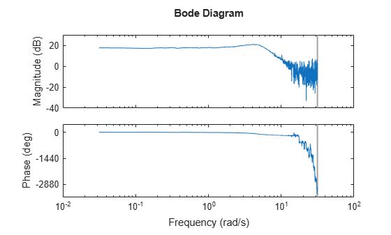
frdata = idfrd(response,W,Ts)
frdata =

IDFRD model.
Contains Frequency Response Data for 1 output(s) and 1 input(s).
Response data is available at 1000 frequency points, ranging from 0.03142 rad/s to 31.42 rad/s.
 
Sample time: 0.1 seconds
Status:                                                         
Created by direct construction or transformation. Not estimated.
 

Plot the data.

bode(frdata)

Figure contains 2 axes objects. Axes object 1 with ylabel Magnitude (dB) contains an object of type line. This object represents frdata. Axes object 2 with ylabel Phase (deg) contains an object of type line. This object represents frdata.

frdata is a complex idfrd object with object properties that you can access using dot notation. For example, confirm the value of Ts.

tsproperty = frdata.Ts
tsproperty = 0.1000

You can also set property values. Set the Name property to 'DC_Converter'.

frdata.Name = 'DC_Converter';

If you import frdata into the System Identification app, the app names this data DC_Converter, and not the variable name frdata.

Use get to obtain the full set of property settings.

get(frdata)
      FrequencyUnit: 'rad/TimeUnit'
             Report: [1x1 idresults.frdest]
       SpectrumData: []
     CovarianceData: []
    NoiseCovariance: []
        InterSample: {'zoh'}
       ResponseData: [1x1x1000 double]
            IODelay: 0
         InputDelay: 0
        OutputDelay: 0
          InputName: {''}
          InputUnit: {''}
         InputGroup: [1x1 struct]
         OutputName: {''}
         OutputUnit: {''}
        OutputGroup: [1x1 struct]
              Notes: [0x1 string]
           UserData: []
               Name: 'DC_Converter'
                 Ts: 0.1000
           TimeUnit: 'seconds'
       SamplingGrid: [1x1 struct]
          Frequency: [1000x1 double]

Convert a state-space model to a frequency response model using the idfrd command.

Load the data z2 and estimate a second-order state-space model sys.

load iddata2 z2
sys = ssest(z2,2);

Convert sys to the idfrd model frsys.
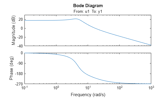
frsys = idfrd(sys)
frsys =

IDFRD model.
Contains Frequency Response Data for 1 output(s) and 1 input(s), and the spectra for disturbances at the outputs.
Response data and disturbance spectra are available at 68 frequency points, ranging from 0.1 rad/s to 1000 rad/s.
 
Output channels: 'y1'
Input channels: 'u1'
Status:                               
Created by conversion from idss model.
 

Plot frsys.

bode(frsys)

Figure contains 2 axes objects. Axes object 1 with title From: u1 To: y1, ylabel Magnitude (dB) contains an object of type line. This object represents frsys. Axes object 2 with ylabel Phase (deg) contains an object of type line. This object represents frsys.

frsys is an idfrd model that you can use as a dynamic system model or as estimation data for a time-domain or frequency-domain model.

Obtain the frequency response of a transfer function model and convert the response into an idfrd object.

Construct a transfer function model with one zero and three poles.

systf = idtf([1 .2],[1 2 1 1]);

Use bode to obtain the frequency response of systf, in terms of magnitude and phase, for the frequency vector f.

f = logspace(-1,1,100);
[mag,phase] = bode(systf,f);

Use the values of mag and phase to compute the complex-valued response response.

response = mag.*exp(1j*phase*pi/180);

Create an idfrd object frdata to store response, specifying a sample rate Ts of 0.8.

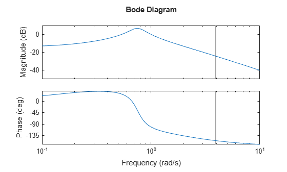
Ts = 0.8;
frdata = idfrd(response,f,Ts)
frdata =

IDFRD model.
Contains Frequency Response Data for 1 output(s) and 1 input(s).
Response data is available at 100 frequency points, ranging from 0.1 rad/s to 10 rad/s.
 
Sample time: 0.8 seconds
Status:                                                         
Created by direct construction or transformation. Not estimated.
 

Plot the data.

bode(frdata)

Figure contains 2 axes objects. Axes object 1 with ylabel Magnitude (dB) contains an object of type line. This object represents frdata. Axes object 2 with ylabel Phase (deg) contains an object of type line. This object represents frdata.

frdata is a complex idfrd object.

Estimate a transfer function model from time-domain data and convert the resulting idtf model to an idfrd model. Estimate a new transfer function model from the frequency response data in the idfrd model. Compare the model responses with the original data.

Load time-domain data z2 and use it to estimate a transfer function sys that has two poles and one zero.

load iddata2 z2
sys = tfest(z2,2,1);

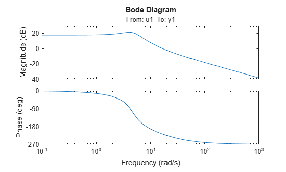
Convert sys to an idfrd model and plot the frequency response.

frsys = idfrd(sys);
bode(sys)

Figure contains 2 axes objects. Axes object 1 with title From: u1 To: y1, ylabel Magnitude (dB) contains an object of type line. This object represents sys. Axes object 2 with ylabel Phase (deg) contains an object of type line. This object represents sys.

Estimate a new transfer function sys1 using the data from frsys as the estimation data.

sys1 = tfest(frsys,2,1);

Compare the responses of sys and sys1 with the original estimation data z2.

compare(z2,sys,sys1)

Figure contains an axes object. The axes object with ylabel y1 contains 3 objects of type line. These objects represent Validation data (y1), sys: 85.71%, sys1: 85.71%.

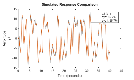
The model responses are identical.

Version History

Introduced before R2006a