Hyperspectral and Multispectral Data Correction
Hyperspectral and multispectral sensors used for remote sensing applications acquire the spectral characteristics of the Earth's surface in many narrow and contiguous bands. When solar radiation is incident on a surface material, the material reflects the incident radiation. The amount of energy reflected signifies the spectral characteristics of the surface material.
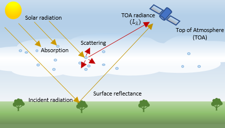
The incident radiation reflected by the surface is known as the surface reflectance. The reflected radiation measured by the sensor positioned at the top of the atmosphere (TOA) is known as the TOA radiance. Ideally, the TOA radiance is equal to the surface reflectance. But, in real conditions, the incident and the reflected radiation are affected by atmospheric phenomena such as scattering and absorption. As a result, the TOA radiance value is the sum of reflections from the surface, reflections from clouds, and scattering from air molecules and aerosol particles in the atmosphere.
Along with the characteristics of the light source and the surface material, the radiation values measured by the sensor are influenced by the sensor gain and bias (offset) at each spectral wavelength. The raw data recorded by the hyperspectral and multispectral sensors is known as the digital numbers (DNs). To use the data for quantitative analysis, you must calibrate the data for TOA radiance values, and estimate the actual surface reflectance values from the DNs. The process of estimating TOA radiance values from the DNs is known as radiometric calibration. The process of estimating the surface reflectance values by removing the atmospheric effects is known as atmospheric correction.
The data recorded by hyperspectral sensors can also be prone to spectral distortions such as the smile effect. The smile effect is caused by a shift in center wavelengths of a band. The smile effect occurs when hyperspectral data contains significant cross-track curvature with nonlinear disturbances along the spectral dimension. These nonlinear disturbances occur only in data captured using push-broom hyperspectral sensors, such as the Hyperion EO-1 and SEBASS.
You can perform radiometric calibration, atmospheric correction, and spectral correction procedures as preprocessing steps for thorough spectral analysis.
Radiometric Calibration
DN to TOA Radiance
To estimate TOA radiance values from DNs, calibrate sensor gain and bias in each spectral band.
Gainλ and Biasλ are the gain and bias values for each spectral band (λ), respectively.
You can find the TOA radiance values for uncalibrated hyperspectral or
multispectral data by using the dn2radiance function. The function reads the gain and the bias
(offset) values for each spectral band from the header file associated with the
data.
TOA Radiance to TOA Reflectance
You can estimate the TOA reflectance values from TOA radiance values. TOA reflectance specifies the ratio of TOA radiance to the radiation incident on the surface.
d is the Earth-sun distance in astronomical units,
ESUNλ is the mean solar irradiance
for each spectral band, and θE is the sun
elevation angle. You can estimate the TOA reflectance values from TOA radiance
values by using the radiance2Reflectance function.
DN to TOA Reflectance
You can directly compute TOA reflectance values from DNs, if the reflectance gain (RGain) and reflectance offset (ROffset) parameters of each spectral band are available.
The dn2reflectance function calibrates the DNs to TOA reflectance values
by using the reflectance gain and offset parameters available in the
metadata.
Atmospheric Correction
Atmospheric correction methods estimate the surface reflectance values from TOA radiance or TOA reflectance values. The atmospheric correction methods are classified as empirical methods and model-based methods.
Empirical methods are scene-based approaches that estimate relative surface reflectance values. Empirical methods are computationally efficient and do not require a priori measurements.
Model-based methods are dependent on in situ atmospheric data and are useful for accurate estimation of surface reflectance values.
| Method | Description |
subtractDarkPixel | Dark pixel subtraction or dark object subtraction, is an empirical method suitable for removing atmospheric haze from hyperspectral and multispectral images. Atmospheric haze is characterized by high DN values, and results in unnatural brightening of the images. The dark pixels are minimum values pixels in each band. Dark pixels are assumed to have zero surface reflectance, and their values account for the additive effect of the atmospheric path radiance. |
empiricalLine | The empirical line calibration method assumes a linear relationship between the surface reflectance and the measured reflectance values. This method assumes that the input hyperspectral data has one or more known target pixels for which the surface reflectance values are available. The calibration method consists of regressing the measured spectral value of the target pixels against the a priori surface reflectance values. You can use the empirical line calibration method if the data is acquired under uniform atmospheric conditions, and the measurements related to the target are time invariant. |
flatField | Flat field correction assumes that the surface being imaged includes a bright, uniform area that has neutral spectral reflectance. The mean spectrum of such an area includes the combined effects of solar irradiance, atmospheric scattering, and absorption. The relative surface reflectance values are estimated by dividing each pixel spectrum by the mean spectrum. |
iarr | Internal average relative reflectance (IARR) is an empirical approach that computes relative surface reflectance by normalizing each pixel spectrum with the mean spectrum. The method assumes that the surface is heterogeneous, and the spectral reflectance characteristics cancel out. As a result, the mean spectrum of the surface is similar to a flat field spectrum. This method is particularly helpful in estimating the relative surface reflectance values for regions without vegetation. |
logResiduals | Logarithmic residual correction of hyperspectral and multispectral data is performed by dividing each pixel spectrum in the data by the spectral geometric mean and the spatial geometric mean. This method is an empirical approach that relies on the statistics of the acquired hyperspectral image. You can use this method to remove solar irradiance and atmospheric transmittance effects. |
sharc | The satellite hypercube atmospheric rapid correction (SHARC) method computes absolute surface reflectance values based on the analytical solutions of the radiative transfer equation. The surface reflectance values are computed by considering the adjacency effect for each point in the surface and the atmospheric effects. You can use this method if the atmospheric model parameters necessary to compute the accurate surface reflectance values are available. |
fastInScene | The fast in-scene method is an empirical approach which performs atmospheric correction based on in-scene characteristics. The method determines correction parameters directly from the pixel spectra of the acquired data. This method results in an approximate correction, but it is computationally faster than model-based methods. Use the fast in-scene method to correct atmospheric effects on hyperspectral and multispectral data with diverse pixel spectra and sufficient number of dark pixels. The method estimates the baseline spectrum by using the dark pixels. |
rrs | Remote sensing reflectance (RRS) for correcting atmospheric effects from hyperspectral and multispectral data containing large water bodies. RRS method estimates the water-leaving radiance and is the atmospheric correction method for ocean color data. |
correctOOB | Out-of-band correction method. This method removes out-of-band (OOB) effects from multispectral data by using the measured radiance and the sensor spectral response values. |
Spectral Correction
You can detect cross-track variation in the oxygen and
carbon-dioxide absorption features, due to a possible smile effect, using the
smileMetric function, which calculates the first derivatives of the
oxygen and carbon-dioxide band images. The first derivative of the adjacent bands is calculated using the absorption band image and the image of the subsequent band , using the equation:
where, is the average FWHM of the two bands and . This derivative calculation is applicable to both the oxygen and
carbon-dioxide absorption band images. The column mean values of the oxygen and
carbon-dioxide derivatives can indicate cross-track nonlinearity caused by the
spectral smile effect. You can reduce the smile effect using the spectral smoothing
or maximum noise fraction (MNF) transform-based method, using the reduceSmile function.
See Also
hypercube | multicube | dn2radiance | dn2reflectance | radiance2Reflectance | correctOOB | empiricalLine | fastInScene | flatField | iarr | logResiduals | rrs | subtractDarkPixel | sharc | smileMetric | reduceSmile