flatField
Apply flat field correction to spectral data
Description
Add-On Required: This feature requires the Hyperspectral Imaging Library for Image Processing Toolbox add-on.
correctedData = flatField(inputData,roi)inputData, using the flat field mean spectrum calculated in the
specified region of interest (ROI) of the data. A valid ROI has these characteristics:
Topographically flat
Spectrally flat (uniform spectral response)
Strong signal source to reduce the impact of random noise
Note
The Hyperspectral Imaging Library for Image Processing Toolbox™ requires desktop MATLAB®, as MATLAB Online™ and MATLAB Mobile™ do not support the library.
Examples
Read hyperspectral data into the workspace.
hcube = imhypercube("paviaU");Display the contrast-stretched RGB color image of the hyperspectral data.
coloredImg = colorize(hcube,Method="rgb",ContrastStretching=true);
figure
imshow(coloredImg)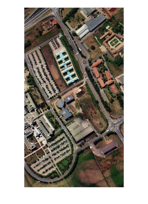
Specify the ROI from which to calculate the flat field mean spectrum.
roi = [1 1 10 10];
Apply the flat field correction to the hyperspectral data.
hcube_flatfield = flatField(hcube,roi);
Read the spectral signature of vegetation from the ECOSTRESS spectral library.
filename = "vegetation.tree.tsuga.canadensis.vswir.tsca-1-47.ucsb.asd.spectrum.txt";
libData = readEcostressSig(filename);
Compute the distance scores of the spectrum of the original hyperspectral data pixels with respect to the reference spectrum.
score = spectralMatch(libData,hcube);
Compute the distance scores of the spectrum of the flat field corrected hyperspectral data pixels with respect to the reference spectrum.
score_flatfield = spectralMatch(libData,hcube_flatfield);
Display the distance scores of the original and the flat field corrected hyperspectral data. The pixels with low distance scores are stronger matches to the reference spectrum, and are more likely to belong to the vegetation region. Observe that the distance scores after flat field correction can differentiate between light vegetation cover and dense vegetation cover.
figure
imagesc([score score_flatfield])
colorbar
title("Original Distance Score | Distance Score after Flat Field Correction")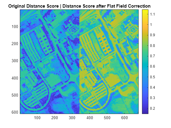
Input Arguments
Output Arguments
References
[1] Roberts, D. A., Y. Yamaguchi, and R. J. P. Lyon. "Comparison of Various Techniques for Calibration of AIS Data." In Proceedings of the Second Airborne Imaging Spectrometer Data Analysis Workshop, ed. Gregg Vane and Alexander F. H. Goetz, 21 -30. Pasadena: Jet Propulsion Laboratory, 1986.
Version History
Introduced in R2020bSee Also
hypercube | multicube | iarr | logResiduals | subtractDarkPixel | empiricalLine | reduceSmile | sharc