sharc
Perform atmospheric correction using satellite hypercube atmospheric rapid correction (SHARC)
Description
Add-On Required: This feature requires the Hyperspectral Imaging Library for Image Processing Toolbox add-on.
newhcube = sharc(hcube)
The input must be radiometrically corrected hyperspectral data. The pixel values of the input data must be either top of atmosphere (TOA) radiance or TOA reflectance values. For better results, use TOA reflectance values.
Note
The Hyperspectral Imaging Library for Image Processing Toolbox™ requires desktop MATLAB®, as MATLAB Online™ and MATLAB Mobile™ do not support the library.
newhcube = sharc(hcube,Name=Value)
Examples
Read a hyperspectral data cube into the workspace.
input = imhypercube("EO1H0440342002212110PY_cropped.dat");Determine the bad spectral band numbers using the BadBands parameter in the metadata.
bandNumber = find(~input.Metadata.BadBands);
Remove the bad spectral bands from the data cube.
input = removeBands(input,BandNumber=bandNumber);
Convert the digital numbers to radiance values by using the dn2radiance function.
hcube = dn2radiance(input);
Convert the radiance values to reflectance values by using the radiance2Reflectance function.
hcube = radiance2Reflectance(hcube);
Compute atmospherically corrected data by using the sharc function.
newhcube = sharc(hcube);
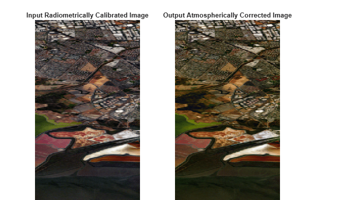
Estimate RGB images of the input and the atmospherically corrected output data. Increase the image contrast by applying contrast stretching.
inputImg = colorize(hcube,Method="rgb",ContrastStretching=true);
outputImg = colorize(newhcube,Method="rgb",ContrastStretching=true);
Display the contrast-stretched RGB images of the input and the atmospherically corrected output data.
figure(Position=[0 0 700 400])
subplot(Position=[0.1 0 0.3 0.9])
imagesc(inputImg)
title("Input Radiometrically Calibrated Image")
axis off
subplot(Position=[0.5 0 0.3 0.9])
imagesc(outputImg)
axis off
title("Output Atmospherically Corrected Image")
Read a hyperspectral data cube into the workspace.
input = imhypercube("EO1H0440342002212110PY_cropped.dat");Determine the bad spectral band numbers using the BadBands parameter in the metadata.
bandNumber = find(~input.Metadata.BadBands);
Remove the bad spectral bands from the data cube.
input = removeBands(input,BandNumber=bandNumber);
Convert the digital numbers to radiance values by using the dn2radiance function.
hcube = dn2radiance(input);
Convert the radiance values to reflectance values by using the radiance2Reflectance function.
hcube = radiance2Reflectance(hcube);
Compute atmospherically corrected data by using the sharc function. Specify the dark pixel location for computing the adjacency effect and the initial atmospheric parameters. The choice of the dark pixel affects the atmospheric correction results.
newhcube = sharc(hcube,DarkPixelLocation=[217 7]);
Estimate RGB images of the input and the atmospherically corrected output data. Increase the image contrast by applying contrast stretching.
inputImg = colorize(hcube,Method="rgb",ContrastStretching=true);
outputImg = colorize(newhcube,Method="rgb",ContrastStretching=true);
Display the contrast-stretched RGB images of the input and the atmospherically corrected output data.
figure(Position=[0 0 700 400])
subplot(Position=[0.1 0 0.3 0.9])
imagesc(inputImg)
title("Input Radiometrically Calibrated Image")
axis off
subplot(Position=[0.5 0 0.3 0.9])
imagesc(outputImg)
axis off
title("Output Atmospherically Corrected Image")
![]()
Input Arguments
Name-Value Arguments
Output Arguments
Limitations
This function does not
support parfor loops, as its performance is already
optimized. (since R2023a)
References
[1] Katkovsky, Leonid, Anton Martinov, Volha Siliuk, Dimitry Ivanov, and Alexander Kokhanovsky. “Fast Atmospheric Correction Method for Hyperspectral Data.” Remote Sensing 10, no. 11 (October 28, 2018): 1698. https://doi.org/10.3390/rs10111698.
Version History
Introduced in R2020b