Linear Regression with Nonpolynomial Terms

You can use linear regression to model the relationship between variables. While some linear regression uses only polynomial terms, you can also use nonpolynomial terms when your data exhibits patterns that polynomials cannot account for.

This example shows how to recognize when nonpolynomial terms are needed, how to build a design matrix, and how to fit a linear regression model with nonpolynomial terms by using the backslash operator (\) (mldivide function). This example also shows how to visualize and validate the model.

Use linear regression with nonpolynomial terms when:

• Polynomial regression does not fit your data well.

• Your data shows rapid growth or decay.

• Your data oscillates.

• Your data flattens out.

Plot Data

Start by plotting your data to identify patterns and decide which terms to include in your model.

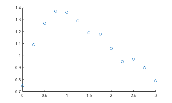
For example, create and visualize a sample predictor variable t and a sample response variable y. The visualization shows that the data grows and then decays over time, suggesting exponential behavior.

t = [0:0.25:3]';
y = [0.75 1.09 1.27 1.37 1.36 1.29 1.19 1.18 1.06 0.95 0.97 0.90 0.79]';
scatter(t,y)

Construct Design Matrix

A design matrix organizes the predictor variables for your data. Each row in the design matrix corresponds to a data point, and each column corresponds to a predictor term.

To construct a design matrix, start by plotting your data and looking for patterns. Then, select predictor functions that reflect those patterns:

• If your data shows rapid growth or decay, consider including exponential terms like exp(t) or exp(-t).

• If your data oscillates, consider including sine or cosine terms like sin(t) or cos(t).

• If your data flattens out, consider including logarithmic terms like log(t).

For this example, because the data shows possible exponential behavior, include these terms in the design matrix:

• Column 1 — Intercept for the constant term

• Column 2 — Exponential decay

• Column 3 — Exponential decay with time scaling

This design matrix represents the equation $a\left(t\right)=a_0+a_1{e}^{-t}+a_{2}t{*e}^{-t}$. For your own data, choose predictor functions that match the patterns in your data.

X = @(t) [ones(size(t)) exp(-t) t.*exp(-t)];

Fit Model

Fit the regression model by solving for the coefficients that minimize the least-squares error by using the \ operator with the design matrix and response data. For more information, see Introduction to Least-Squares Fitting (Curve Fitting Toolbox).

a = X(t)\y

a = 3×1

    0.4836
    0.2700
    2.0612

Display the fitted model.

model = a(1) + " + " + a(2) + "*exp(-t) + "  + a(3) + "*t*exp(-t)"

model = 
"0.48362 + 0.27*exp(-t) + 2.0612*t*exp(-t)"

If the model needs improvement, consider adding terms to or removing terms from the design matrix.

Evaluate and Visualize Model

To visualize a model, first evaluate the model at query points and return the predicted response values. Then visualize the data and the model.

For example, get the response values for the model over a finer range of t values.

tQuery = [0:0.01:3]';
yFit = X(tQuery) * a;

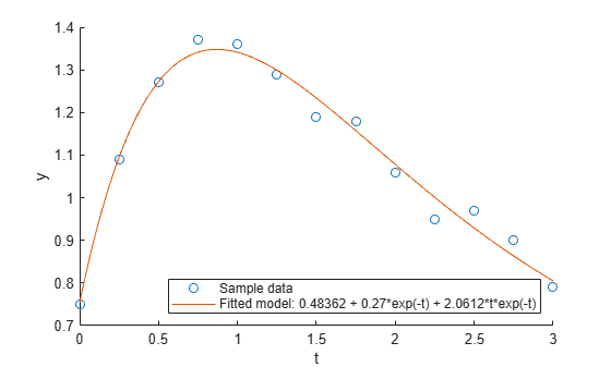
Then visualize the sample data and the model.

scatter(t,y)
hold on
plot(tQuery,yFit)
hold off
xlabel("t")
ylabel("y")
legend("Sample data",["Fitted model: " + model],Location="southeast")

Validate Model

Validate the model by computing the largest error between the model predictions and the sample data.

Find the times that are common in both your sample data and the model prediction times. Then, create a vector of the model predictions for those common times to directly compare to the observed data.

TF = ismember(tQuery,t);
yFit_t = yFit(TF)

yFit_t = 13×1

    0.7536
    1.0952
    1.2725
    1.3414
    1.3412
    1.2991
    1.2337
    1.1574
    1.0781
    1.0009
    0.9288
    0.8632
    0.8049

Calculate the maximum absolute difference between the observed data and the model predictions at those common times. A small maximum error relative to the data values indicates a good fit.

maxError = max(abs(y - yFit_t))

maxError = 
0.0509