Time Series Objects and Collections

Open Live Script

The recommended way to store time series data is with timetable, which has a broad set of supporting functions for preprocessing, restructuring, and analysis. To get started with timetables, see Create Timetables.

Some existing code uses these objects, described in this topic:

timeseries — Stores numeric data and time values, as well as the metadata information that includes units, events, data quality, and interpolation method.
tscollection — Stores a collection of timeseries objects that share a common time vector, convenient for performing operations on synchronized time series with different units.

Data Samples in `timeseries`

Consider data that consists of three sensor signals: two signals represent the position of an object in meters, and the third represents its velocity in meters/second. NaN represents a missing data value.

x = [-0.2 -0.3 13;
     -0.1 -0.4 15;
      NaN  2.8 17;
      0.5 0.3 NaN;
     -0.3 -0.1 15];

The first two columns of x contain quantities with the same units, and you can create a multivariate timeseries object to store these two time series.

ts_pos = timeseries(x(:,1:2),1:5,"name","Position")

  timeseries

  Common Properties:
            Name: 'Position'
            Time: [5x1 double]
        TimeInfo: [1x1 tsdata.timemetadata]
            Data: [5x2 double]
        DataInfo: [1x1 tsdata.datametadata]

  More properties, Methods

A data sample consists of one or more values associated with a specific time in the timeseries object. The number of data samples in a time series is the same as the length of the time vector, which is 5 in this example. To find the size of the data sample, use getdatasamplesize.

getdatasamplesize(ts_pos)

ans = 1×2

     1     2

You can create a second timeseries object to store the velocity data.

ts_vel = timeseries(x(:,3),1:5,"name","Velocity");

If you want to perform operations on ts_pos and ts_vel while keeping them synchronized, group them in a collection. For more information, see Time Series Collections.

Creating Time Series Objects

The sample data in count.dat has 24 rows and three columns. Each column represents hourly vehicle counts at each of three town intersections.

Load the data and create three timeseries objects to store the data collected at each intersection.

load count.dat
count1 = timeseries(count(:,1),1:24,"name","Intersection1");
count2 = timeseries(count(:,2),1:24,"name","Intersection2");
count3 = timeseries(count(:,3),1:24,"name","Intersection3");

Alternatively, when all time series have the same data units and you want to keep them synchronized during calculations, create a single object.

count_ts = timeseries(count,1:24,"name","traffic_counts");

Modifying Units and Interpolation Method

By default, a time series has a time vector with units of seconds and a start time of 0 sec, and the series uses linear interpolation.

Modify the time units to be hours for the three time series.

count1.TimeInfo.Units = "hours";
count2.TimeInfo.Units = "hours";
count3.TimeInfo.Units = "hours";

Change the data units for count1 to cars.

count1.DataInfo.Units = "cars";

Set the interpolation method for count1 to zero-order hold. The other time series use the default method, linear interpolation.

count1.DataInfo.Interpolation = tsdata.interpolation("zoh");

View the modified data properties.

count1.DataInfo

  tsdata.datametadata
  Namespace: tsdata

  Common Properties:
               Units: 'cars'
       Interpolation: zoh (tsdata.interpolation)

  More properties, Methods

Defining Events

Events mark the data at specific times. Events also provide a convenient way to synchronize multiple time series.

Add two events to each series that mark the times of the AM commute and PM commute.

e1 = tsdata.event("AMCommute",8);
e1.Units = "hours";            
count1 = addevent(count1,e1);  
count2 = addevent(count2,e1);  
count3 = addevent(count3,e1);  

e2 = tsdata.event("PMCommute",18);
e2.Units = "hours";            
count1 = addevent(count1,e2);  
count2 = addevent(count2,e2);  
count3 = addevent(count3,e2);

Plot the first time series. Red circle markers indicate the events.

plot(count1)

Figure contains an axes object. The axes object with title Time Series Plot:Intersection1, xlabel Time (hours), ylabel Intersection1 (cars) contains 2 objects of type stair, line. One or more of the lines displays its values using only markers

Time Series Collections

A collection is a group of synchronized time series. The time vectors of the timeseries objects in a collection must match. Each individual time series in a collection is called a member. Typically, you use collections for time series that have different data units. In this simple example, all time series have the same units.

tsc = tscollection({count1,count2,count3},"name","count_coll")

Time Series Collection Object: count_coll

Time vector characteristics

      Start time            1 hours
      End time              24 hours

Member Time Series Objects:

      Intersection1
      Intersection2
      Intersection3

Resampling a Collection

A resampling operation is used to either select existing data at specific time values, or to interpolate data at finer intervals. If the new time vector contains time values that did not exist in the previous time vector, the new data values are calculated using the interpolation method associated with each time series.

Resample the time series to include data values every two hours instead of every hour and save it as a new tscollection object.

tsc1 = resample(tsc,1:2:24);

In some cases, you might need a finer sampling of information than you currently have and it is reasonable to obtain it by interpolating data values. For instance, interpolate values at each half-hour mark.

tsc1 = resample(tsc,1:0.5:24);

The new data points in Intersection1 are calculated by using the zero-order hold interpolation method, which holds the value of the previous sample constant. Plot the members of tsc1 with markers to see the results of interpolating.

plot(tsc1.Intersection1,"-x")

The new data points in Intersection2 use linear interpolation, the default method.

plot(tsc1.Intersection2,"-o")

Figure contains an axes object. The axes object with title Time Series Plot:Intersection2, xlabel Time (hours), ylabel Intersection2 contains 2 objects of type line. One or more of the lines displays its values using only markers

Adding a Data Sample to a Collection

Add a data sample to the first collection member at 3.25 hours.

tsc1 = addsampletocollection(tsc1,"time",3.25,"Intersection1",5);

The time series includes values for every half hour, so the new value is the sixth element.

tsc1.Intersection1.Data

Because you did not specify the data values for Intersection2 and Intersection3 in the new sample, the missing values are represented by NaN for these members.

tsc1.Intersection2.Data

Handling Missing Data

The Intersection2 and Intersection3 members in the tsc1 collection currently contain missing values at 3.25 hours, represented by NaN. Before analyzing this data, you can either remove the missing values or use interpolation to replace them.

For instance, find and remove the data samples that contain NaN values. For each missing value in Intersection2, the data at that time is removed from all members of the collection.

tsc2 = delsamplefromcollection(tsc1,"index",... 
       find(isnan(tsc1.Intersection2.Data)));

Alternatively, replace the NaN values in Intersection2 and Intersection3 by resampling using interpolation. The default interpolation method for these time series is linear interpolation.

tsc1 = resample(tsc1,tsc1.Time);
tsc1.Intersection2.Data

Plotting Collection Members

To plot data in a time series collection, plot its members one at a time.

Optionally, to display the time vectors as formatted dates and times, specify the start date. In this case, the time units are hours, so you can specify a display format that shows hours and minutes.

tsc1.TimeInfo.StartDate = "25-DEC-2022 00:00:00";
tsc1.TimeInfo.Format = "HH:MM";

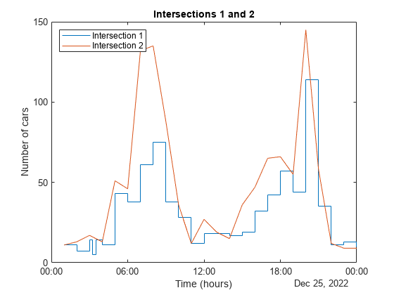
When you plot a single member of a collection, its time units display on the x-axis and its data units display on the y-axis. The plot title is displayed as Time Series Plot:<member name>.

If you specify hold on before plotting multiple members of the collection, no annotations display. The time series plot method does not attempt to show labels and titles on held figures because the descriptors for the series can be different. To preserve date formatting, hold after plotting the first member. Update the title and labels to reflect the entire collection.

plot(tsc1.Intersection1,"Displayname","Intersection 1")
hold on  
plot(tsc1.Intersection2,"Displayname","Intersection 2")

legend("Location","NorthWest")
title("Intersections 1 and 2")
xlabel("Time (hours)")
ylabel("Number of cars")
hold off

Figure contains an axes object. The axes object with title Intersections 1 and 2, xlabel Time (hours), ylabel Number of cars contains 2 objects of type stair, line. These objects represent Intersection 1, Intersection 2.