DDE of Neutral Type
This example shows how to use ddensd to solve a neutral DDE (delay differential equation), where delays appear in derivative terms. The problem was originally presented by Paul [1].
The equation is
.
The history function is for .
Since the equation has time delays in a term, the equation is called a neutral DDE. If the time delays are only present in terms, then the equation would be a constant or state-dependent DDE, depending on what form the time delays have.
To solve this equation in MATLAB®, you need to code the equation, delays, and history before calling the delay differential equation solver ddensd. You either can include these as local functions at the end of a file (as done here), or save them as separate files in a directory on the MATLAB path.
Code Delays
First, write functions to define the delays in the equation. The first term in the equation with a delay is .
function dy = dely(t,y)
    dy = t/2;
end
The other term in the equation with a delay is .
function dyp = delyp(t,y)
    dyp = t-pi;
end
In this example, only one delay for and one delay for are present. If there were more delays, then you can add them in these same function files, so that the functions return vectors instead of scalars.
Note: All functions are included as local functions at the end of the example.
Code Equation
Now, create a function to code the equation. This function should have the signature yp = ddefun(t,y,ydel,ypdel), where:
tis time (independent variable).yis the solution (dependent variable).ydelcontains the delays for .ypdelcontains the delays for .
These inputs are automatically passed to the function by the solver, but the variable names determine how you code the equation. In this case:
ydelypdel
function yp = ddefun(t,y,ydel,ypdel)
    yp = 1 + y - 2*ydel^2 - ypdel;
end
Code Solution History
Next, create a function to define the solution history. The solution history is the solution for times .
function y = history(t)
    y = cos(t);
end
Solve Equation
Finally, define the interval of integration and solve the DDE using the ddensd solver.
tspan = [0 pi];
sol = ddensd(@ddefun, @dely, @delyp, @history, [0,pi]);
Plot Solution
The solution structure sol has the fields sol.x and sol.y that contain the internal time steps taken by the solver and corresponding solutions at those times. However, you can use deval to evaluate the solution at the specific points.
Evaluate the solution at 20 equally spaced points between 0 and pi.
tn = linspace(0,pi,20);
yn = deval(sol,tn);
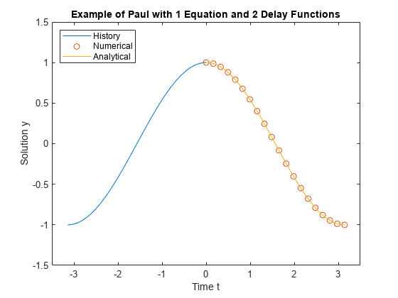
Plot the calculated solution and history against the analytical solution.
th = linspace(-pi,0);
yh = history(th);
ta = linspace(0,pi);
ya = cos(ta);

plot(th,yh,tn,yn,'o',ta,ya)
legend('History','Numerical','Analytical','Location','NorthWest')
xlabel('Time t')
ylabel('Solution y')
title('Example of Paul with 1 Equation and 2 Delay Functions')
axis([-3.5 3.5 -1.5 1.5])
Local Functions
Listed here are the local helper functions that the DDE solver ddensd calls to calculate the solution. Alternatively, you can save these functions as their own files in a directory on the MATLAB path.
function yp = ddefun(t,y,ydel,ypdel) % equation being solved
    yp = 1 + y - 2*ydel^2 - ypdel;
end
%-------------------------------------------
function dy = dely(t,y) % delay for y
    dy = t/2;
end
%-------------------------------------------
function dyp = delyp(t,y) % delay for y'
    dyp = t-pi;
end
%-------------------------------------------
function y = history(t) % history function for t < 0
    y = cos(t);
end
%-------------------------------------------
References
[1] Paul, C.A.H. “A Test Set of Functional Differential Equations.” Numerical Analysis Reports. No. 243. Manchester, UK: Math Department, University of Manchester, 1994.
See Also
ddensd | ddesd | dde23 | deval