solve

Solve ODE over interval or at specified points

Since R2023b

Syntax

S = solve(F,t)

S = solve(F,t0,tf)

S = solve(F,t0,tf,Refine=N)

Description

S = solve(F,t) computes the solution for the ODE represented by F at the specified time values in the vector t. "Time" refers to the independent variable in the ODE problem.

S = solve(F,t0,tf) computes the solution in the time interval [t0 tf], returning the solution at each step chosen by the solver.

S = solve(F,t0,tf,Refine=N) additionally specifies the number of evenly spaced solution values for each solver step.

Examples

Solve ODE Problem at Specified Times

Create an ode object to integrate the function dydt = @(t,y) (1/2)*t^2. Specify the initial value of dydt as 0.

F = ode(ODEFcn=@(t,y) (1/2)*t^2,InitialValue=0);

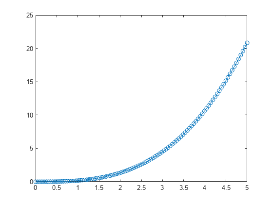
Integrate the ode object by using the solve method. Specify a vector of times using linspace to evaluate the solution at specific time points in the interval [0 5].

t = linspace(0,5);
S = solve(F,t)

S = 
  ODEResults with properties:

        Time: [0 0.0505 0.1010 0.1515 0.2020 0.2525 0.3030 0.3535 0.4040 0.4545 0.5051 0.5556 0.6061 0.6566 0.7071 0.7576 0.8081 0.8586 0.9091 0.9596 1.0101 1.0606 1.1111 1.1616 1.2121 1.2626 1.3131 1.3636 1.4141 1.4646 1.5152 1.5657 ... ] (1x100 double)
    Solution: [0 2.1471e-05 1.7177e-04 5.7972e-04 0.0014 0.0027 0.0046 0.0074 0.0110 0.0157 0.0215 0.0286 0.0371 0.0472 0.0589 0.0725 0.0879 0.1055 0.1252 0.1473 0.1718 0.1988 0.2286 0.2612 0.2968 0.3355 0.3774 0.4226 0.4713 0.5237 ... ] (1x100 double)

Plot the results.

plot(S.Time,S.Solution,"-o")

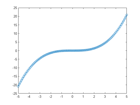
Integrate the ode object again, this time specifying time points in the interval [-5 5]. Even though the initial value of dydt is applied at F.InitialTime=0 by default, the solve method can evaluate the solution before the initial time.

t2 = linspace(-5,5);
S2 = solve(F,t2);
plot(S2.Time,S2.Solution,"-o")

Solve ODE over Time Interval

Create an ode object to integrate this system of equations.

$$\begin{array}{l}{y}_1^{\prime }=y_2\\ y_2^{\prime }=-y_1\end{array}$$

Specify initial values of ${\mathit{y}}_1=0$ and ${\mathit{y}}_2=1$.

F = ode(ODEFcn=@(t,y) [y(2); -y(1)],InitialValue=[0 1]);

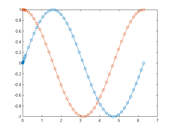
Integrate the ode object over the interval [0 2*pi] by using the solve method. Plot the results.

S = solve(F,0,2*pi);
plot(S.Time,S.Solution,"-o")

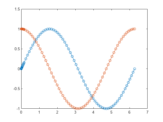
Integrate the ode object again, this time specifying Refine=6 to generate additional solution points in each time step.

S2 = solve(F,0,2*pi,Refine=6);
plot(S2.Time,S2.Solution,"-o")

Input Arguments

F — ODE problem to solve

ode object

ODE problem to solve, specified as an ode object.

t — Time points to compute solution

real vector

Time points to compute solution, specified as a vector with real elements. The solver returns the solution evaluated at the given time points. However, the solver does not step precisely to each point specified in t. Instead, the solver uses its own internal steps to compute the solution, and then evaluates the solution at the requested points in t. The solutions produced at the specified points are of the same order of accuracy as the solutions computed at each internal step.

The time points you specify in t are not bound by the value of the InitialTime property of the ode object F. You can specify time values before or after the value of InitialTime.

The solver uses the values in t to calculate suitable values for the F.SolverOptions.InitialStep and F.SolverOptions.MaxStep options:

• The specified time points give an indication of the scale for the problem, which can affect the value of InitialStep used by the solver. Therefore, specifying the initial and final time points of the interval with t0,tf can lead to different integration results compared to specifying a vector of times.

• The solver uses the initial and final time points to calculate the maximum step size MaxStep. Therefore, changing the initial or final values in t can cause the solver to use a different step sequence, which might change the solution.

Example: S = solve(F,1:10) solves the ODE problem represented by F at the time points 1:10.

t0,tf — Interval of integration

real scalars

Interval of integration, specified as two real scalars that indicate the initial (t0) and final (tf) time points. The solver returns the solution evaluated at each internal integration step within the specified time interval.

The time points you specify in t0 and tf are not bound by the value of the InitialTime property of the ode object F. You can specify time values before or after the value of InitialTime.

The solver uses the initial and final time points to calculate the maximum step size F.SolverOptions.MaxStep. Therefore, changing t0 or tf can cause the solver to use a different step sequence, which might change the solution.

Example: S = solve(F,1,10) solves the ODE problem represented by F in the interval [1 10].

N — Solution refinement factor

scalar integer

Solution refinement factor, specified as a scalar integer. The scalar specifies a factor by which the number of output points should increase in each step.

The default value of N for most solvers is 1, but ode45 uses a default value of 4, while ode78 and ode89 use a default value of 8. These solvers use a larger default value to compensate for their tendency to take large steps.

• If the refinement factor is 1, then the solver returns solutions only at the end of each step.

• If the refinement factor is greater than 1, then the solver subdivides each step into N smaller intervals and returns solutions at each point.

The extra values produced by the refinement factor are computed by means of continuous extension formulas. The solvers use these specialized formulas to obtain accurate solutions between computed time steps without significant increase in computation time.

Example: S = solve(F,1,10,Refine=5) solves the ODE problem represented by F in the interval [1 10] and returns 5 points per time step.

Output Arguments

S — Computed solution

ODEResults object

Computed solution, returned as an ODEResults object.

Version History

Introduced in R2023b