Cette page a été traduite par traduction automatique. Cliquez ici pour voir la dernière version en anglais.

optimize

Optimiser le graphique du facteur

Depuis R2022a

Syntaxe

solnInfo = optimize(graph)

solnInfo = optimize(graph,poseNodeIDs)

solnInfo = optimize(___,solverOptions)

Description

La fonction optimize optimise un graphe factoriel pour trouver une solution qui minimise le coût du problème des moindres carrés non linéaires formulé par le graphe factoriel.

solnInfo = optimize(graph) optimise le graphique de facteurs à l'aide des options de solveur par défaut, définit les états des nœuds sur les états optimisés et renvoie les informations de solution résultantes.

solnInfo = optimize(graph,poseNodeIDs) optimise les nœuds de pose spécifiés et tous les nœuds associés, à l'exception des nœuds de pose non spécifiés.

Remarque

Les ID de nœud spécifiés forment un graphique de facteurs connectés. Pour plus d’informations, consultez Connectivité du graphique factoriel.

solnInfo = optimize(___,solverOptions) optimise le graphe de facteurs à l'aide des options spécifiées du solveur de graphe de facteurs, en plus de toute combinaison d'arguments d'entrée des syntaxes précédentes.

Exemples

Optimiser le graphique à facteurs simples

Créez un graphique factoriel.

fg = factorGraph;

Définissez deux états de pose approximatifs du robot.

rstate = [0 0 0;
          1 1 pi/2];

Définissez la mesure de pose relative entre deux nœuds de l'odométrie comme la différence de pose entre les états avec du bruit. La mesure relative doit être dans le référentiel du deuxième nœud, vous devez donc faire pivoter la différence de position pour être dans le référentiel du deuxième nœud.

posediff = diff(rstate);
rotdiffso2 = so2(posediff(3),"theta");
transformedPos = transform(inv(rotdiffso2),posediff(1:2));
odomNoise = 0.1*rand;
measure = [transformedPos posediff(3)] + odomNoise;

Créez un facteur à deux poses SE(2) avec la mesure relative. Ajoutez ensuite le facteur au graphique des facteurs pour créer deux nœuds.

ids = generateNodeID(fg,1,"factorTwoPoseSE2");
f = factorTwoPoseSE2(ids,Measurement=measure);
addFactor(fg,f);

Obtenez l'état des deux nœuds de pose.

stateDefault = nodeState(fg,ids)

stateDefault = 2×3

     0     0     0
     0     0     0

Ces nœuds étant nouveaux, ils ont des valeurs d’état par défaut. Idéalement, avant d'optimiser, vous devez attribuer une estimation approximative de la pose absolue. Cela augmente la possibilité pour la fonction optimize de trouver le minimum global. Sinon, optimize pourrait se retrouver piégé dans le minimum local, produisant une solution sous-optimale.

Conservez le premier état du nœud à l'origine et définissez le deuxième état du nœud sur une position xy approximative à [0.9 0.95] et une rotation thêta de pi/3 radians. Dans des applications pratiques, vous pouvez utiliser les mesures des capteurs de votre odométrie pour déterminer l'état approximatif de chaque nœud de pose.

nodeState(fg,ids(2),rstate(2,:))

ans = 1×3

    1.0000    1.0000    1.5708

Avant d'optimiser, enregistrez l'état du nœud afin de pouvoir le réoptimiser si nécessaire.

statePriorOpt1 = nodeState(fg,ids);

Optimisez les nœuds et vérifiez les états des nœuds.

optimize(fg);
stateOpt1 = nodeState(fg,ids)

stateOpt1 = 2×3

   -0.1038    0.8725    0.1512
    1.1038    0.1275    1.8035

Notez qu'après optimisation, le premier nœud n'est pas resté à l'origine car bien que le graphe ait l'estimation initiale de l'état, le graphe n'a aucune contrainte sur la position absolue. Le graphique n'a que la mesure de pose relative, qui agit comme une contrainte pour la pose relative entre les deux nœuds. Le graphique tente donc de réduire le coût lié à la pose relative, mais pas à la pose absolue. Pour fournir plus d'informations au graphique, vous pouvez fixer l'état des nœuds ou ajouter un facteur de mesure préalable absolu.

Réinitialisez les états, puis corrigez le premier nœud. Vérifiez ensuite que le premier nœud est fixe.

nodeState(fg,ids,statePriorOpt1);
fixNode(fg,ids(1))
isNodeFixed(fg,ids(1))

ans = logical
   1

Réoptimisez le graphique des facteurs et obtenez les états des nœuds.

optimize(fg)

ans = struct with fields:
             InitialCost: 1.8470
               FinalCost: 1.8470e-16
      NumSuccessfulSteps: 2
    NumUnsuccessfulSteps: 0
               TotalTime: 8.6069e-05
         TerminationType: 0
        IsSolutionUsable: 1
        OptimizedNodeIDs: 1
            FixedNodeIDs: 0

stateOpt2 = nodeState(fg,ids)

stateOpt2 = 2×3

         0         0         0
    1.0815   -0.9185    1.6523

Notez qu'après optimisation de ce temps, l'état du premier nœud est resté à l'origine.

Optimiser progressivement le graphique des facteurs à l'aide d'une fenêtre coulissante

Lors de la création de grands graphiques factoriels, il est inefficace de réoptimiser l’intégralité d’un graphique factoriel chaque fois que vous ajoutez de nouveaux facteurs et nœuds au graphique à un nouveau pas de temps. Cet exemple montre une approche d'optimisation alternative. Au lieu d'optimiser un graphique de facteurs entier à chaque pas de temps, optimisez un sous-ensemble ou une fenêtre des nœuds de pose les plus récents. Ensuite, au pas de temps suivant, faites glisser la fenêtre vers l'ensemble suivant de nœuds de pose les plus récents et optimisez ces nœuds de pose. Cette approche minimise le nombre de fois où vous devez réoptimiser les anciennes parties du graphique factoriel.

Créez un graphique factoriel et chargez le fichier sensorData MAT. Ce fichier MAT contient des données de capteur pour dix pas de temps.

fg = factorGraph;
load sensorData.mat

Définissez la taille de la fenêtre sur cinq nœuds de pose. Plus la taille de la fenêtre glissante est grande, plus l’optimisation devient précise. Si la taille de la fenêtre glissante est petite, il se peut qu’il n’y ait pas suffisamment de mesures pour que l’optimisation produise une solution précise.

windowSize = 5;

Pour chaque pas de temps :

1. Générez un nouvel ID de nœud pour le nœud de pose du pas de temps actuel.

2. Obtenez les données de pose actuelles pour le pas de temps actuel.

3. Générez un ID de nœud pour un nœud de point de repère nouvellement détecté. Connectez le nœud de pose actuel à deux points de repère. Supposons que le premier point de repère que le robot détecte au pas de temps actuel est le même que le deuxième point de repère que le robot a détecté au pas de temps précédent. Pour le premier pas de temps, les deux points de repère sont nouveaux, vous devez donc générer deux ID de point de repère.

4. Ajoutez un facteur à deux poses qui connecte le nœud de pose au pas de temps actuel avec le nœud de pose du pas de temps précédent.

5. Ajoutez des facteurs de repère qui créent les ID de nœud de point de repère spécifiés au graphique.

6. Définissez l’état initial des nœuds de points de repère et du nœud de pose actuel comme données de capteur pour le pas de temps actuel.

7. Si le graphique contient au moins cinq nœuds de pose, corrigez le nœud de pose le plus ancien dans la fenêtre glissante, puis optimisez les nœuds de pose dans la fenêtre glissante. Étant donné que les mesures entre les poses et les mesures entre les poses et les points de repère sont relatives, vous devez corriger le nœud le plus ancien, sinon la solution issue de l'optimisation risque d'être incorrecte. Notez que lorsque vous spécifiez les nœuds de pose, cela inclut des facteurs qui associent les nœuds de pose spécifiés à d'autres nœuds de pose spécifiés ou à tout nœud sans pose.

for t = 1:10
    % 1. Generate node ID for pose at this time step
    currPoseID = generateNodeID(fg,1);
    % 2. Get current pose data at this time step
    currPose = poseInitStateData{t};

    % 3. On the first time step, create pose node and two landmarks
    if t == 1
        lmID = generateNodeID(fg,2);
        lmFactorIDs = [currPoseID lmID(1); 
                       currPoseID lmID(2)];
    else % On subsequent time steps, connect to previous landmark and create new landmark
        lmIDNew = generateNodeID(fg,1);
        allLandmarkIDs = nodeIDs(fg,NodeType="POINT_XY");
        lmIDPrior = allLandmarkIDs(end);
        lmID = [lmIDPrior lmIDNew];
        lmFactorIDs = [currPoseID lmIDPrior; 
                       currPoseID lmIDNew];
    end

    % 4. After first time step, connect current pose with previous node
    if t > 1
        allPoseIDs = nodeIDs(fg,NodeType="POSE_SE2");
        prevPoseID = allPoseIDs(end);
        poseFactor = factorTwoPoseSE2([prevPoseID currPoseID],Measurement=poseSensorData{t});
        addFactor(fg,poseFactor);
    end

    % 5. Create landmark factors with sensor observation data and add to graph
    lmFactor = factorPoseSE2AndPointXY(lmFactorIDs,Measurement=lmSensorData{t});
    addFactor(fg,lmFactor);

    % 6. Set initial guess for states of the pose node and observed landmarks nodes
    nodeState(fg,lmID,lmInitStateData{t});
    nodeState(fg,currPoseID,currPose);
    
    % 7. Optimize nodes in sliding window when there are enough poses
    if t >= windowSize
        allPoseIDs = nodeIDs(fg,NodeType="POSE_SE2");
        poseIDsInWindow = allPoseIDs(end-(windowSize-1):end);
        fixNode(fg,poseIDsInWindow(1));
        optimize(fg,poseIDsInWindow);
    end
end

Obtenez tous les identifiants de pose et tous les identifiants de points de repère. Utilisez ces identifiants pour obtenir l’état optimisé des nœuds de pose et des nœuds de points de repère.

allPoseIDs = nodeIDs(fg,NodeType="POSE_SE2");
allLandmarkIDs = nodeIDs(fg,NodeType="POINT_XY");
optPoseStates = nodeState(fg,allPoseIDs);
optLandmarkStates = nodeState(fg,allLandmarkIDs);

Utilisez la fonction d'assistance exampleHelperPlotPositionsAndLandmarks pour tracer à la fois la vérité terrain des poses et des points de repère.

initPoseStates = cat(1,poseInitStateData{:});
initLandmarkStates = cat(1,lmInitStateData{:});
exampleHelperPlotPositionsAndLandmarks(initPoseStates, ...
                                       initLandmarkStates)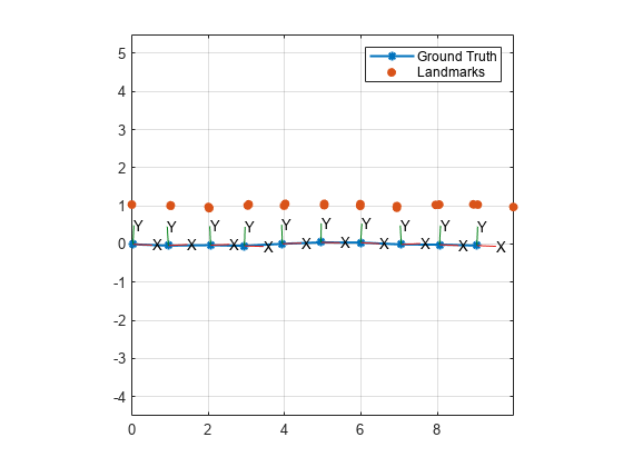

Tracez la vérité terrain des poses et des points de repère ainsi que la solution d'optimisation.

exampleHelperPlotPositionsAndLandmarks(initPoseStates, ...
                                       initLandmarkStates, ...
                                       optPoseStates, ...
                                       optLandmarkStates)

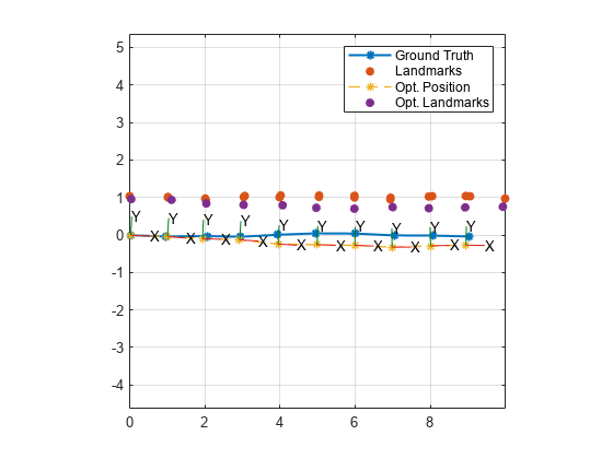
Notez que vous pouvez améliorer la précision de l'optimisation en augmentant la taille de la fenêtre glissante ou en utilisant les options personnalisées du solveur de graphe factoriel.

Arguments d'entrée

graph — Graphique factoriel

Objet factorGraph

Graphique factoriel, spécifié comme objet factorGraph .

poseNodeIDs — ID des nœuds de pose à optimiser

N - vecteur de ligne d'éléments d'entiers non négatifs

ID des nœuds de pose à optimiser dans le graphe de facteurs, spécifiés comme un vecteur de ligne d'éléments N d'entiers non négatifs. N est le nombre total de nœuds de pose à optimiser.

Les nœuds de pose spécifiés par poseNodeIDs doivent tous être de type "POSE_SE2", ou doivent tous être de type "POSE_SE3". Les nœuds de pose spécifiés doivent également être uniques. Par exemple, poseNodeIDs ne peut pas être [1 2 1] car l'ID de nœud 1 n'est pas unique dans ce vecteur.

Les nœuds de pose spécifiés dans le graphe de facteurs doivent former un graphe de facteurs connecté. Pour plus d’informations, consultez Connectivité du graphique factoriel.

solverOptions — Options du solveur pour le graphique de facteurs

Objet factorGraphSolverOptions

Options du solveur pour le graphique factoriel, spécifié comme objet factorGraphSolverOptions .

Arguments de sortie

solnInfo — Résultats de l'optimisation

structure

Résultats de l'optimisation, renvoyés sous forme de structure contenant :

• InitialCost — Coût initial du problème des moindres carrés non linéaires formulé par le graphe factoriel avant l'optimisation.

• FinalCost — Coût final du problème des moindres carrés non linéaires formulé par le graphe factoriel après l'optimisation.

  Remarque

  Le coût est la somme des termes d’erreur, appelés résidus, où chaque résidu est fonction d’un sous-ensemble de mesures factorielles.

• NumSuccessfulSteps — Nombre d'itérations au cours desquelles le solveur diminue le coût. Cette valeur inclut l'itération d'initialisation à 0 en plus des itérations de minimisation.

• NumUnsuccessfulSteps — Nombre d'itérations dans lesquelles l'itération est numériquement invalide ou le solveur ne diminue pas le coût.

• TotalTime — Temps total d'optimisation du solveur en secondes.

• TerminationType — Type de terminaison sous forme d'entier compris dans la plage [0, 2] :

  • 0 — Le solveur a trouvé une solution qui répond au critère de convergence et réduit les coûts après optimisation.

  • 1 — Le solveur n'a pas pu trouver de solution répondant au critère de convergence après avoir exécuté le nombre maximal d'itérations.

  • 2 — Le solveur s'est arrêté en raison d'une erreur.

• IsSolutionUsable — La solution est utilisable si la solution a convergé ou si optimize a atteint le nombre maximum d'itérations. La valeur est 1 (true) si la solution est utilisable et la valeur est 0 (false) si la solution n'est pas utilisable.

• OptimizedNodeIDs — ID de nœud des nœuds optimisés lors de l'optimisation.

• FixedNodeIDs — ID de nœud des nœuds qui ont été corrigés lors de l'optimisation dans le graphe de facteurs ou le graphe de facteurs partiel. Notez que ces nœuds fixes contribuent toujours à l'optimisation des autres nœuds spécifiés.

En savoir plus

Connectivité du graphique factoriel

Un graphe factoriel est considéré comme connecté s’il existe un chemin entre chaque paire de nœuds. Par exemple, pour un graphe de facteurs contenant quatre nœuds de pose, connectés consécutivement par trois facteurs, il existe des chemins dans le graphe de facteurs allant d'un nœud du graphique à n'importe quel autre nœud du graphique.

connected = isConnected(fg,[1 2 3 4])

connected =

     1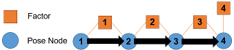

Si le graphe ne contient pas le nœud 3, bien qu'il existe toujours un chemin du nœud 1 au nœud 2, il n'y a pas de chemin du nœud 1 ou du nœud 2 au nœud 4.

connected = isConnected(fg,[1 2 4])

connected =

     0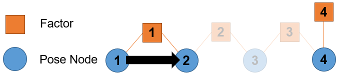

Un graphique factoriel entièrement connecté est important pour l’optimisation. Si le graphique factoriel n'est pas entièrement connecté, l'optimisation se produit séparément pour chacun des graphiques déconnectés, ce qui peut produire des résultats indésirables. La connectivité des graphiques peut devenir plus complexe lorsque vous spécifiez certains sous-ensembles d'ID de nœud de pose à optimiser. En effet, la fonction optimize optimise des parties du graphique de facteurs en utilisant les ID spécifiés pour identifier les facteurs à utiliser pour créer un graphique de facteurs partiel. optimize ajoute un facteur au graphique de facteur partiel si ce facteur se connecte à l'un des nœuds de pose spécifiés et ne se connecte à aucun nœud de pose non spécifié. La fonction ajoute également tous les nœuds non posés auxquels les facteurs ajoutés se connectent, mais n'ajoute pas d'autres facteurs connectés à ces nœuds. Par exemple, pour ce graphique de facteurs, il existe trois nœuds de pose, deux nœuds sans pose et les facteurs qui relient les nœuds.

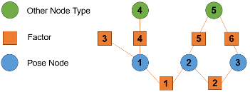
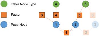
Si vous spécifiez les nœuds 1 et 2, les facteurs 1, 3, 4 et 5 forment un graphique de facteurs pour l'optimisation car ils se connectent aux nœuds de pose 1 et 2. L'optimisation inclut les nœuds 4 et 5 car ils se connectent à des facteurs liés aux ID de nœud de pose spécifiés.

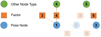
Si vous spécifiez poseNodeIDs comme [1 3], alors la fonction optimize optimise chaque graphe séparé séparément car le graphe de facteurs formé ne contient pas de chemin. entre les nœuds 1 et 3.

Conseils

• Avant d'optimiser le graphique de facteurs ou un sous-ensemble de nœuds, utilisez la fonction nodeState pour enregistrer les états des nœuds dans l'espace de travail. Si, après avoir exécuté l'optimisation, vous souhaitez y apporter des ajustements, vous pouvez redéfinir les états des nœuds sur les états enregistrés.

• Pour déboguer une optimisation partielle d'un graphique de facteurs, vérifiez les champs OptimizedNodeIDs et FixedNodeIDs de l'argument de sortie solnInfo pour voir lequel des les ID de nœud optimisés et lesquels des nœuds fixes ont contribué à l'optimisation.

• Pour vérifier si poseNodeIDs forme un graphe de facteurs connexe, utilisez la fonction isConnected .

Capacités étendues

Génération de code C/C++
Générez du code C et C++ avec MATLAB® Coder™.

Historique des versions

Introduit dans R2022a

R2023b: Optimiser les nœuds spécifiés

La fonction optimize prend désormais en charge la spécification des ID de nœud pour optimiser un sous-ensemble de nœuds à partir d'un graphe de facteurs. Ceci est utile pour des applications telles que Visual SLAM, où vous devez optimiser les nœuds dans une fenêtre glissante.

Voir aussi

Objets

• factorGraph | factorGraphSolverOptions

Rubriques

• Landmark SLAM Using AprilTag Markers