pdeplot3D
Plot solution or surface mesh for 3-D problem
Syntax
Description
pdeplot3D(results.Mesh,ColorMapData=results.VonMisesStress,Deformation=results.Displacement)
plots the von Mises stress and shows the deformed shape for a 3-D structural
analysis problem.
pdeplot3D(results.Mesh,ColorMapData=results.Temperature)
plots the temperature at nodal locations for a 3-D thermal analysis
problem.
pdeplot3D(results.Mesh,ColorMapData=results.ElectricPotential)
plots the electric potential at nodal locations for a 3-D electrostatic analysis
problem.
pdeplot3D(results.Mesh,ColorMapData=results.NodalSolution)
plots the solution at nodal locations.
pdeplot3D( plots the surface
mesh specified in model)model. This syntax does not work with an
femodel object.
pdeplot3D(___,
plots the surface mesh, the data at nodal locations, or both the mesh and data,
depending on the Name,Value)Name,Value pair arguments. Use any
arguments from the previous syntaxes.
h = pdeplot3D(___)
Examples
Create an femodel object for static structural analysis and include the geometry of a beam.
model = femodel(AnalysisType="structuralStatic", ...
                Geometry="SquareBeam.stl");
Plot the geometry.
pdegplot(model.Geometry,FaceLabels="on",FaceAlpha=0.5)
Specify Young's modulus and Poisson's ratio.
model.MaterialProperties = ...
    materialProperties(PoissonsRatio=0.3, ...
                       YoungsModulus=210E3);
Specify that face 6 is a fixed boundary.
model.FaceBC(6) = faceBC(Constraint="fixed");Specify the surface traction for face 5.
model.FaceLoad(5) = faceLoad(SurfaceTraction=[0;0;-2]);
Generate a mesh and solve the problem.
model = generateMesh(model);
R = solve(model);
Plot the deformed shape with the von Mises stress using the default scale factor. By default, pdeplot3D internally determines the scale factor based on the dimensions of the geometry and the magnitude of deformation.
figure
pdeplot3D(R.Mesh, ...
          ColorMapData=R.VonMisesStress, ...
          Deformation=R.Displacement)

Plot the same results with the scale factor 500.
figure
pdeplot3D(R.Mesh, ...
          ColorMapData=R.VonMisesStress, ...
          Deformation=R.Displacement, ...
          DeformationScaleFactor=500)

Plot the same results without scaling.
figure
pdeplot3D(R.Mesh, ...
          ColorMapData=R.VonMisesStress)
Evaluate the von Mises stress in a beam under a harmonic excitation.
Create and plot a beam geometry.
gm = multicuboid(0.06,0.005,0.01);
pdegplot(gm,FaceLabels="on",FaceAlpha=0.5)
view(50,20)
Create an femodel for transient structural analysis and include the geometry.
model = femodel(AnalysisType="structuralTransient", ...
                Geometry=gm);
Specify Young's modulus, Poisson's ratio, and the mass density of the material.
model.MaterialProperties = ...
    materialProperties(YoungsModulus=210E9, ...
                       PoissonsRatio=0.3, ...
                       MassDensity=7800);
Fix one end of the beam.
model.FaceBC(5) = faceBC(Constraint="fixed");Apply a sinusoidal displacement along the y-direction on the end opposite the fixed end of the beam.
yDisplacementFunc = ...
@(location,state) ones(size(location.y))*1E-4*sin(50*state.time);
model.FaceBC(3) = faceBC(YDisplacement=yDisplacementFunc);
Generate a mesh.
model = generateMesh(model,Hmax=0.01);
Specify the zero initial displacement and velocity.
model.CellIC = cellIC(Displacement=[0;0;0],Velocity=[0;0;0]);
Solve the model.
tlist = 0:0.002:0.2;
R = solve(model,tlist);
Evaluate the von Mises stress in the beam.
vmStress = evaluateVonMisesStress(R);
Plot the von Mises stress for the last time-step.
figure
pdeplot3D(R.Mesh,ColorMapData = vmStress(:,end))
title("von Mises Stress in the Beam for the Last Time-Step")
Solve a 3-D steady-state thermal problem.
Create an femodel object for a steady-state thermal problem and include a geometry representing a block.
model = femodel(AnalysisType="thermalSteady", ...
                Geometry="Block.stl");
Plot the block geometry.
pdegplot(model.Geometry, ...
         FaceLabels="on", ...
         FaceAlpha=0.5)
axis equal

Assign material properties.
model.MaterialProperties = ...
    materialProperties(ThermalConductivity=80);
Apply a constant temperature of 100 °C to the left side of the block (face 1) and a constant temperature of 300 °C to the right side of the block (face 3). All other faces are insulated by default.
model.FaceBC(1) = faceBC(Temperature=100);
model.FaceBC(3) = faceBC(Temperature=300);
Mesh the geometry and solve the problem.
model = generateMesh(model);
thermalresults = solve(model)
thermalresults =
  SteadyStateThermalResults with properties:

    Temperature: [12822×1 double]
     XGradients: [12822×1 double]
     YGradients: [12822×1 double]
     ZGradients: [12822×1 double]
           Mesh: [1×1 FEMesh]
The solver finds the temperatures and temperature gradients at the nodal locations. To access these values, use thermalresults.Temperature, thermalresults.XGradients, and so on. For example, plot temperatures at the nodal locations.
pdeplot3D(thermalresults.Mesh,ColorMapData=thermalresults.Temperature)

For a 3-D steady-state thermal problem, evaluate heat flux at the nodal locations and at the points specified by x, y, and z coordinates.
Create an femodel object for steady-state thermal analysis and include a block geometry in the model.
model = femodel(AnalysisType="thermalSteady", ...
                Geometry="Block.stl");
Plot the geometry.
pdegplot(model.Geometry,FaceLabels="on",FaceAlpha=0.5)
title("Copper block, cm")
axis equal

Assuming that this is a copper block, the thermal conductivity of the block is approximately .
model.MaterialProperties = ...
    materialProperties(ThermalConductivity=4);
Apply a constant temperature of 373 K to the left side of the block (face 1) and a constant temperature of 573 K to the right side of the block (face 3).
model.FaceBC(1) = faceBC(Temperature=373);
model.FaceBC(3) = faceBC(Temperature=573);
Apply a heat flux boundary condition to the bottom of the block.
model.FaceLoad(4) = faceLoad(Heat=-20);
Mesh the geometry and solve the problem.
model = generateMesh(model);
R = solve(model)
R =
  SteadyStateThermalResults with properties:

    Temperature: [12822×1 double]
     XGradients: [12822×1 double]
     YGradients: [12822×1 double]
     ZGradients: [12822×1 double]
           Mesh: [1×1 FEMesh]
Evaluate heat flux at the nodal locations.
[qx,qy,qz] = evaluateHeatFlux(R);

figure
pdeplot3D(R.Mesh,FlowData=[qx qy qz])

Create a grid specified by x, y, and z coordinates, and evaluate heat flux to the grid.
[X,Y,Z] = meshgrid(1:26:100,1:6:20,1:11:50);

[qx,qy,qz] = evaluateHeatFlux(R,X,Y,Z);
Reshape the qx, qy, and qz vectors, and plot the resulting heat flux.
qx = reshape(qx,size(X));
qy = reshape(qy,size(Y));
qz = reshape(qz,size(Z));
figure
quiver3(X,Y,Z,qx,qy,qz)

Alternatively, you can specify the grid by using a matrix of query points.
querypoints = [X(:) Y(:) Z(:)]';
[qx,qy,qz] = evaluateHeatFlux(R,querypoints);

qx = reshape(qx,size(X));
qy = reshape(qy,size(Y));
qz = reshape(qz,size(Z));
figure
quiver3(X,Y,Z,qx,qy,qz)

Solve an electromagnetic problem and find the electric potential and field distribution for a 3-D geometry representing a plate with a hole.
Create an femodel object for electrostatic analysis and include a geometry representing a plate with a hole.
model = femodel(AnalysisType="electrostatic", ...
                Geometry="PlateHoleSolid.stl");
Plot the geometry.
pdegplot(model.Geometry,FaceLabels="on",FaceAlpha=0.3)
Specify the vacuum permittivity in the SI system of units.
model.VacuumPermittivity = 8.8541878128E-12;
Specify the relative permittivity of the material.
model.MaterialProperties = ...
    materialProperties(RelativePermittivity=1);
Specify the charge density for the entire geometry.
model.CellLoad = cellLoad(ChargeDensity=5E-9);
Apply the voltage boundary conditions on the side faces and the face bordering the hole.
model.FaceBC(3:6) = faceBC(Voltage=0);
model.FaceBC(7) = faceBC(Voltage=1000);
Generate the mesh.
model = generateMesh(model);
Solve the model.
R = solve(model)
R =
  ElectrostaticResults with properties:

      ElectricPotential: [4747×1 double]
          ElectricField: [1×1 FEStruct]
    ElectricFluxDensity: [1×1 FEStruct]
                   Mesh: [1×1 FEMesh]
Plot the electric potential.
figure
pdeplot3D(R.Mesh,ColorMapData=R.ElectricPotential)

Plot the electric field.
pdeplot3D(R.Mesh,FlowData=[R.ElectricField.Ex ...
                           R.ElectricField.Ey ...
                           R.ElectricField.Ez])

Plot a PDE solution on the geometry surface. First, create a PDE model and import a 3-D geometry file. Specify boundary conditions and coefficients. Mesh the geometry and solve the problem.
model = createpde;
importGeometry(model,"Block.stl");
applyBoundaryCondition(model,"dirichlet",Face=1:4,u=0);
specifyCoefficients(model,m=0,d=0,c=1,a=0,f=2);
generateMesh(model);
results = solvepde(model)
results =
  StationaryResults with properties:

    NodalSolution: [12822×1 double]
       XGradients: [12822×1 double]
       YGradients: [12822×1 double]
       ZGradients: [12822×1 double]
             Mesh: [1×1 FEMesh]
Plot the solution at the nodal locations on the geometry surface.
u = results.NodalSolution;
msh = results.Mesh;
pdeplot3D(msh,ColorMapData=u)

Since R2026a
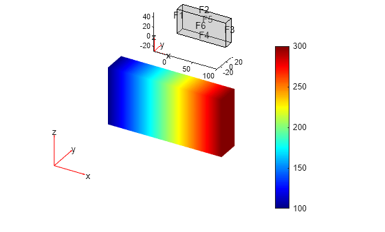
Position two Axes objects in a figure. Add the solution plot to one object and the geometry plot to another object.
Solve a 3-D steady-state thermal problem on a block geometry.
model = femodel(AnalysisType="thermalSteady", ...
                Geometry="Block.stl");
model.MaterialProperties = ...
    materialProperties(ThermalConductivity=80);
model.FaceBC(1) = faceBC(Temperature=100);
model.FaceBC(3) = faceBC(Temperature=300);
model = generateMesh(model);
R = solve(model);
Specify the position of the first Axes object so that it has a lower left corner at the point (0.1 0.1) with a width and height of 0.7. Specify the position of the second Axes object so that it has a lower left corner at the point (0.35 0.7) with a width and height of 0.3. By default, the values are normalized to the figure. Return the Axes objects as ax1 and ax2.
ax1 = axes(Position=[0.1 0.1 0.7 0.7]);
ax2 = axes(Position=[0.35 0.7 0.3 0.3]);
Plot the temperature distribution and the geometry adding the temperature distribution plot to ax1 and the geometry plot to ax2.
pdeplot3D(ax1,R.Mesh,ColorMapData=R.Temperature)
pdegplot(ax2,model.Geometry, ...
             FaceLabels="on", ...
             FaceAlpha=0.3)
Import a geometry and generate a linear mesh.
gm = fegeometry("Tetrahedron.stl");
gm = generateMesh(gm,Hmax=20,GeometricOrder="linear");
Plot the mesh.
mesh = gm.Mesh;
pdeplot3D(mesh)

Alternatively, you can use the nodes and elements of the mesh as input arguments for pdeplot3D.
pdeplot3D(mesh.Nodes,mesh.Elements)

Display the node labels on the surface of a simple mesh.
pdeplot3D(mesh,NodeLabels="on")
view(101,12)
Display the element labels.
pdeplot3D(mesh,ElementLabels="on")
view(101,12)