pdeplot
Plot solution or mesh for 2-D problem
Syntax
Description
pdeplot(results.Mesh,XYData=results.Temperature,ColorMap="hot")
plots the temperature at nodal locations for a 2-D thermal analysis problem.
This syntax creates a colored surface plot using the "hot"
colormap.
pdeplot(results.Mesh,XYData=results.VonMisesStress,Deformation=results.Displacement)
plots the von Mises stress and shows the deformed shape for a 2-D structural
analysis problem.
pdeplot(results.Mesh,XYData=results.ModeShapes.ux) plots
the x-component of the modal displacement for a 2-D
structural modal analysis problem.
pdeplot(results.Mesh,XYData=results.ElectricPotential)
plots the electric potential at nodal locations for a 2-D electrostatic analysis
problem.
pdeplot(results.Mesh,XYData=results.NodalSolution) plots
the solution at nodal locations as a colored surface plot using the default
colormap.
pdeplot( plots the mesh
specified in model)model. This syntax does not work with an
femodel object.
pdeplot(___,
plots the mesh, the data at the nodal locations, or both the mesh and the data,
using the Name,Value)Name,Value pair arguments. Use any arguments from
the previous syntaxes.
Specify at least one of the FlowData (vector field plot),
XYData (colored surface plot), or
ZData (3-D height plot) name-value pairs. You can
combine any number of plot types.
For a thermal analysis, you can plot temperature or gradient of temperature.
For a structural analysis, you can plot displacement, stress, strain, and von Mises stress. In addition, you can show the deformed shape and specify the scaling factor for the deformation plot.
For an electromagnetic analysis, you can plot electric or magnetic potentials, fields, and flux densities.
Examples
Solve a 2-D transient thermal problem.
Create a geometry representing a square plate with a diamond-shaped region in its center.
SQ1 = [3; 4; 0; 3; 3; 0; 0; 0; 3; 3];
D1 = [2; 4; 0.5; 1.5; 2.5; 1.5; 1.5; 0.5; 1.5; 2.5];
gd = [SQ1 D1];
sf = 'SQ1+D1';
ns = char('SQ1','D1');
ns = ns';
g = decsg(gd,sf,ns);
pdegplot(g,EdgeLabels="on",FaceLabels="on")
xlim([-1.5 4.5])
ylim([-0.5 3.5])
axis equal

Create an femodel object for transient thermal analysis and include the geometry.
model = femodel(AnalysisType="thermalTransient", ...
                Geometry=g);
For the square region, assign these thermal properties:
Thermal conductivity is
Mass density is
Specific heat is
model.MaterialProperties(1) = ...
    materialProperties(ThermalConductivity=10, ...
                       MassDensity=2, ...
                       SpecificHeat=0.1);
For the diamond region, assign these thermal properties:
Thermal conductivity is
Mass density is
Specific heat is
model.MaterialProperties(2) = ...
    materialProperties(ThermalConductivity=2, ...
                       MassDensity=1, ...
                       SpecificHeat=0.1);
Assume that the diamond-shaped region is a heat source with a density of .
model.FaceLoad(2) = faceLoad(Heat=4);
Apply a constant temperature of 0 °C to the sides of the square plate.
model.EdgeBC(1:4) = edgeBC(Temperature=0);
Set the initial temperature to 0 °C.
model.FaceIC = faceIC(Temperature=0);
Generate the mesh.
model = generateMesh(model);
The dynamics for this problem are very fast. The temperature reaches a steady state in about 0.1 second. To capture the most active part of the dynamics, set the solution time to logspace(-2,-1,10). This command returns 10 logarithmically spaced solution times between 0.01 and 0.1.
tlist = logspace(-2,-1,10);
Solve the equation.
thermalresults = solve(model,tlist);
Plot the solution with isothermal lines by using a contour plot.
T = thermalresults.Temperature;
msh = thermalresults.Mesh;
pdeplot(msh,XYData=T(:,10),Contour="on",ColorMap="hot")
axis equal

Create an femodel object for structural analysis and include the unit square geometry in the model.
model = femodel(AnalysisType="structuralStatic", ...
                Geometry=@squareg);
Plot the geometry.
pdegplot(model.Geometry,EdgeLabels="on")
xlim([-1.1 1.1])
ylim([-1.1 1.1])
Specify Young's modulus and Poisson's ratio.
model.MaterialProperties = ...
    materialProperties(PoissonsRatio=0.3, ...
                       YoungsModulus=210E3);
Specify the x-component of the enforced displacement for edge 1.
model.EdgeBC(1) = edgeBC(XDisplacement=0.001);
Specify that edge 3 is a fixed boundary.
model.EdgeBC(3) = edgeBC(Constraint="fixed");Generate a mesh and solve the problem.
model = generateMesh(model);
R = solve(model);
Plot the deformed shape using the default scale factor. By default, pdeplot internally determines the scale factor based on the dimensions of the geometry and the magnitude of deformation.
pdeplot(R.Mesh, ...
        XYData=R.VonMisesStress, ...
        Deformation=R.Displacement, ...
        ColorMap="jet")
axis equal

Plot the deformed shape with the scale factor 500.
pdeplot(R.Mesh, ...
        XYData=R.VonMisesStress, ...
        Deformation=R.Displacement, ...
        DeformationScaleFactor=500,...
        ColorMap="jet")
axis equal

Plot the deformed shape without scaling.
pdeplot(R.Mesh, ...
        XYData=R.VonMisesStress, ...
        ColorMap="jet")
axis equal

Find the fundamental (lowest) mode of a 2-D cantilevered beam, assuming prevalence of the plane-stress condition.
Specify geometric and structural properties of the beam, along with a unit plane-stress thickness.
length = 5;
height = 0.1;
E = 3E7;
nu = 0.3;
rho = 0.3/386;
Create a geometry.
gdm = [3;4;0;length;length;0;0;0;height;height];
g = decsg(gdm,'S1',('S1')');
Create an femodel object for modal structural analysis and include the geometry.
model = femodel(Analysistype="structuralModal", ...
                Geometry=g);
Define a maximum element size (five elements through the beam thickness).
hmax = height/5;
Generate a mesh.
model=generateMesh(model,Hmax=hmax);
Specify the structural properties and boundary constraints.
model.MaterialProperties = ...
    materialProperties(YoungsModulus=E, ...
                       MassDensity=rho, ...
                       PoissonsRatio=nu);
model.EdgeBC(4) = edgeBC(Constraint="fixed");
Compute the analytical fundamental frequency (Hz) using the beam theory.
I = height^3/12;
analyticalOmega1 = 3.516*sqrt(E*I/(length^4*(rho*height)))/(2*pi)
analyticalOmega1 =
126.9498
Specify a frequency range that includes an analytically computed frequency and solve the model.
R = solve(model,FrequencyRange=[0,1e6])
R =
  ModalStructuralResults with properties:

    NaturalFrequencies: [32×1 double]
            ModeShapes: [1×1 FEStruct]
                  Mesh: [1×1 FEMesh]
The solver finds natural frequencies and modal displacement values at nodal locations. To access these values, use R.NaturalFrequencies and R.ModeShapes.
R.NaturalFrequencies/(2*pi)
ans = 32×1
105 ×

    0.0013
    0.0079
    0.0222
    0.0433
    0.0711
    0.0983
    0.1055
    0.1462
    0.1930
    0.2455
    0.2948
    0.3034
    0.3664
    0.4342
    0.4913
      ⋮
R.ModeShapes
ans =
  FEStruct with properties:

           ux: [6511×32 double]
           uy: [6511×32 double]
    Magnitude: [6511×32 double]
Plot the y-component of the solution for the fundamental frequency.
pdeplot(R.Mesh,XYData=R.ModeShapes.uy(:,1))
title(['First Mode with Frequency ', ...
        num2str(R.NaturalFrequencies(1)/(2*pi)),' Hz'])
axis equal

Solve an electromagnetic problem and find the electric potential and field distribution for a 2-D geometry representing a plate with a hole.
Create an femodel object for electrostatic analysis and include a geometry representing a plate with a hole.
model = femodel(AnalysisType="electrostatic",...
                Geometry="PlateHolePlanar.stl");
Plot the geometry with edge labels.
pdegplot(model.Geometry,EdgeLabels="on")
Specify the vacuum permittivity value in the SI system of units.
model.VacuumPermittivity = 8.8541878128E-12;
Specify the relative permittivity of the material.
model.MaterialProperties = ...
    materialProperties(RelativePermittivity=1);
Apply the voltage boundary conditions on the edges framing the rectangle and the circle.
model.EdgeBC(1:4) = edgeBC(Voltage=0);
model.EdgeBC(5) = edgeBC(Voltage=1000);
Specify the charge density for the entire geometry.
model.FaceLoad = faceLoad(ChargeDensity=5E-9);
Generate the mesh.
model = generateMesh(model);
Solve the model.
R = solve(model)
R =
  ElectrostaticResults with properties:

      ElectricPotential: [1231×1 double]
          ElectricField: [1×1 FEStruct]
    ElectricFluxDensity: [1×1 FEStruct]
                   Mesh: [1×1 FEMesh]
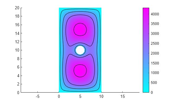
Plot the electric potential distribution using the Contour parameter to display equipotential lines and the Levels parameter to specify how many equipotential lines to display.
pdeplot(R.Mesh,XYData=R.ElectricPotential, ...
               Contour="on", ...
               Levels=5)
axis equal

You can also use the Levels parameter to specify electric potential values for which to display equipotential lines.
pdeplot(R.Mesh,XYData=R.ElectricPotential, ...
               Contour="on", ...
               Levels=[500 1500 2500 4000])
axis equal

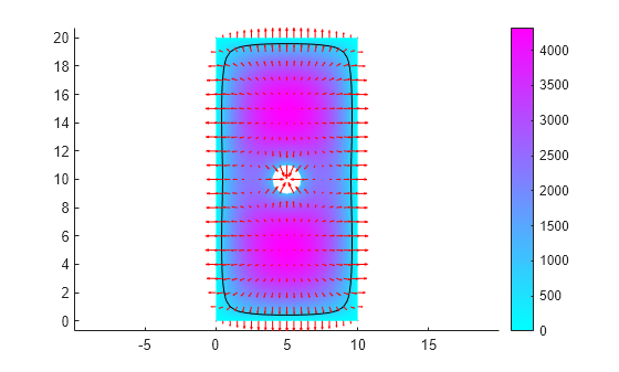
Now plot the electric potential, the equipotential line for the potential value 750, and a quiver plot representing the electric field.
pdeplot(R.Mesh,XYData=R.ElectricPotential, ...
               Contour="on", ...
               Levels=[750 750], ...
               FlowData=[R.ElectricField.Ex ...
                         R.ElectricField.Ey])
axis equal

Create colored 2-D and 3-D plots of a solution to a PDE model.
Create a PDE model. Include the geometry of the built-in function lshapeg. Mesh the geometry.
model = createpde;
geometryFromEdges(model,@lshapeg);
generateMesh(model);
Set the zero Dirichlet boundary conditions on all edges.
applyBoundaryCondition(model,"dirichlet", ...
                             Edge=1:model.Geometry.NumEdges, ...
                             u=0);
Specify the coefficients and solve the PDE.
specifyCoefficients(model,m=0, ...
                          d=0, ...
                          c=1, ...
                          a=0, ...
                          f=1);
results = solvepde(model)
results =
  StationaryResults with properties:

    NodalSolution: [1141×1 double]
       XGradients: [1141×1 double]
       YGradients: [1141×1 double]
       ZGradients: []
             Mesh: [1×1 FEMesh]
Plot the 2-D solution at the nodal locations.
u = results.NodalSolution;
msh = results.Mesh;
pdeplot(msh,XYData=u)
axis equal
Plot the 3-D solution.
pdeplot(msh,XYData=u,ZData=u)

Plot the gradient of a PDE solution as a quiver plot.
Create a PDE model. Include the geometry of the built-in function lshapeg. Mesh the geometry.
model = createpde;
geometryFromEdges(model,@lshapeg);
generateMesh(model);
Set the zero Dirichlet boundary conditions on all edges.
applyBoundaryCondition(model,"dirichlet", ...
                             Edge=1:model.Geometry.NumEdges, ...
                             u=0);
Specify coefficients and solve the PDE.
specifyCoefficients(model,m=0, ...
                          d=0, ...
                          c=1, ...
                          a=0, ...
                          f=1);
results = solvepde(model)
results =
  StationaryResults with properties:

    NodalSolution: [1141×1 double]
       XGradients: [1141×1 double]
       YGradients: [1141×1 double]
       ZGradients: []
             Mesh: [1×1 FEMesh]
Plot the gradient of the solution at the nodal locations as a quiver plot.
ux = results.XGradients;
uy = results.YGradients;
msh = results.Mesh;
pdeplot(msh,FlowData=[ux,uy])
axis equal
Plot the solution of a 2-D PDE in 3-D with the "jet" coloring and a mesh, and include a quiver plot. Get handles to the axes objects.
Create a PDE model. Include the geometry of the built-in function lshapeg. Mesh the geometry.
model = createpde;
geometryFromEdges(model,@lshapeg);
generateMesh(model);
Set zero Dirichlet boundary conditions on all edges.
applyBoundaryCondition(model,"dirichlet", ...
                             Edge=1:model.Geometry.NumEdges, ...
                             u=0);
Specify coefficients and solve the PDE.
specifyCoefficients(model,m=0, ...
                          d=0, ...
                          c=1, ...
                          a=0, ...
                          f=1);
results = solvepde(model)
results =
  StationaryResults with properties:

    NodalSolution: [1141×1 double]
       XGradients: [1141×1 double]
       YGradients: [1141×1 double]
       ZGradients: []
             Mesh: [1×1 FEMesh]
Plot the solution in 3-D with the "jet" coloring and a mesh, and include the gradient as a quiver plot.
u = results.NodalSolution;
ux = results.XGradients;
uy = results.YGradients;
msh = results.Mesh;
h = pdeplot(msh,XYData=u,ZData=u, ...
                FaceAlpha=0.5, ...
                FlowData=[ux,uy], ...
                ColorMap="jet", ...
                Mesh="on");

Since R2026a
Position two Axes objects in a figure. Add the solution plot to one object and the geometry plot to another object.
Solve a heat transfer problem on the unit square geometry.
model = femodel(AnalysisType="thermalSteady", ...
    Geometry=@squareg);
model.MaterialProperties = ...
    materialProperties(ThermalConductivity=1);
model.EdgeBC(3) = edgeBC(Temperature=100);
model.EdgeLoad(1) = edgeLoad(Heat=-10);
model = generateMesh(model);
results = solve(model);
Specify the position of the first Axes object so that it has a lower left corner at the point (0.1 0.1) with a width and height of 0.7. Specify the position of the second Axes object so that it has a lower left corner at the point (0.4 0.65) with a width and height of 0.3. By default, the values are normalized to the figure. Return the Axes objects as ax1 and ax2.
ax1 = axes(Position=[0.1 0.1 0.7 0.7]);
ax2 = axes(Position=[0.4 0.65 0.3 0.3]);

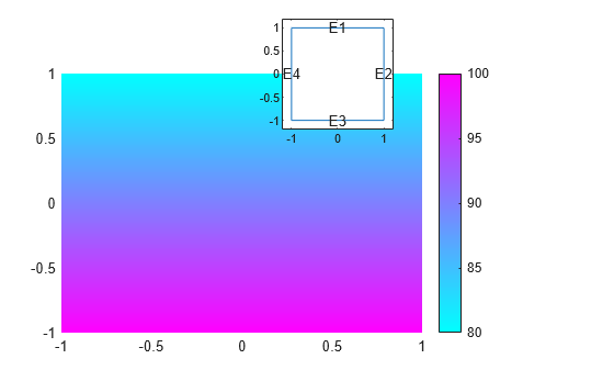
Plot the temperature distribution and the geometry adding the temperature distribution plot to ax1 and the geometry plot to ax2.
pdeplot(ax1,results.Mesh,XYData=results.Temperature)
pdegplot(ax2,model.Geometry,EdgeLabels="on")
xlim(ax2,[-1.2 1.2])
ylim(ax2,[-1.2 1.2])
Create an femodel object and include the geometry of the built-in function lshapeg.
model = femodel(Geometry=@lshapeg);
Generate and plot the mesh.
model = generateMesh(model,Hmax=0.3, ...
                     GeometricOrder="linear");
msh = model.Geometry.Mesh;
pdeplot(msh)

Alternatively, you can use the nodes and elements of the mesh as input arguments for pdeplot.
pdeplot(msh.Nodes,msh.Elements)

Display the node labels.
pdeplot(msh,NodeLabels="on")
Display the element labels.
pdeplot(msh,ElementLabels="on")
Input Arguments
Mesh description, specified as an FEMesh object.
Nodal coordinates, specified as a 2-by-NumNodes matrix. NumNodes is the number of nodes.
Element connectivity matrix in terms of the node IDs, specified as a 3-by-NumElements or 6-by-NumElements matrix. Linear meshes contain only corner nodes. For linear meshes, the connectivity matrix has three nodes per 2-D element. Quadratic meshes contain corner nodes and nodes in the middle of each edge of an element. For quadratic meshes, the connectivity matrix has six nodes per 2-D element.
Model object, specified as a PDEModel object.
Mesh points, specified as a 2-by-Np matrix of points, where
Np is the number of points in the mesh. For a description of the
(p,e,t) matrices, see Mesh Data as [p,e,t] Triples.
Typically, you use the p, e, and t
data exported from the PDE Modeler app, or generated by initmesh or refinemesh.
Example: [p,e,t] = initmesh(gd)
Data Types: double
Mesh edges, specified as a 7-by-Ne matrix of edges,
where Ne is the number of edges in the mesh. For a description of the
(p,e,t) matrices, see Mesh Data as [p,e,t] Triples.
Typically, you use the p, e, and t
data exported from the PDE Modeler app, or generated by initmesh or refinemesh.
Example: [p,e,t] = initmesh(gd)
Data Types: double
Mesh triangles, specified as a 4-by-Nt matrix of
triangles, where Nt is the number of triangles in the mesh. For a
description of the (p,e,t)
matrices, see Mesh Data as [p,e,t] Triples.
Typically, you use the p, e, and t
data exported from the PDE Modeler app, or generated by initmesh or refinemesh.
Example: [p,e,t] = initmesh(gd)
Data Types: double
Since R2026a
Target axes for a plot, specified as a handle to a MATLAB
Axes object. See Axes Properties.
Name-Value Arguments
Specify optional pairs of arguments as
Name1=Value1,...,NameN=ValueN, where Name is
the argument name and Value is the corresponding value.
Name-value arguments must appear after other arguments, but the order of the
pairs does not matter.
Before R2021a, use commas to separate each name and value, and enclose
Name in quotes.
Example: pdeplot(results.Mesh,XYData=u,ZData=u)
Tip
Specify at least one of the FlowData (vector field plot),
XYData (colored surface plot), or
ZData (3-D height plot) name-value pairs. Otherwise,
pdeplot plots the mesh with no data.
Data Plots
Colored surface plot data, specified as a vector. If you use a
[p,e,t] representation, specify data for points
in a vector of length size(p,2), or specify data for
triangles in a vector of length size(t,2).
Typically, you set
XYDatato the solutionu. Thepdeplotfunction usesXYDatafor coloring both 2-D and 3-D plots.pdeplotuses the colormap specified in theColorMapname-value pair, using the style specified in theXYStylename-value pair.When the
Contourname-value pair is"on",pdeplotalso plots level curves ofXYData.pdeplotplots the real part of complex data.
To plot the kth component of a solution to a PDE
system, extract the relevant part of the solution, for example:
results = solvepde(model);
u = results.NodalSolution; % each column of u has one component of u
pdeplot(results.Mesh,XYData=u(:,k)) % data for column k
Example: XYData=u
Data Types: double
Coloring choice, specified as one of the following values:
"off"— No shading, only mesh is displayed."flat"— Each triangle in the mesh has a uniform color."interp"— Plot coloring is smoothly interpolated.
The coloring choice relates to the XYData
name-value pair.
Example: XYStyle="flat"
Data Types: char | string
Data for the 3-D plot heights, specified as a matrix. If you use a
[p,e,t] representation, provide data for points
in a vector of length size(p,2) or data for triangles
in a vector of length size(t,2).
Typically, you set
ZDatatou, the solution. TheXYDataname-value pair sets the coloring of the 3-D plot.The
ZStylename-value pair specifies whether the plot is continuous or discontinuous.pdeplotplots the real part of complex data.
To plot the kth component of a solution to a PDE
system, extract the relevant part of the solution, for example:
results = solvepde(model);
u = results.NodalSolution; % each column of u has one component of u
pdeplot(results.Mesh,XYData=u(:,k),ZData=u(:,k)) % data for column k
Example: ZData=u
Data Types: double
3-D plot style, specified as one of these values:
"off"— No 3-D plot."discontinuous"— Each triangle in the mesh has a uniform height in a 3-D plot."continuous"— 3-D surface plot is continuous.
If you use ZStyle without specifying the
ZData name-value pair, then
pdeplot ignores
ZStyle.
Example: ZStyle="discontinuous"
Data Types: char | string
Data for the quiver plot,
specified as an M-by-2 matrix,
where M is the number of mesh nodes.
FlowData contains the x and
y values of the field at the mesh points.
When you use ZData to represent a 2-D PDE solution
as a 3-D plot and you also include a quiver plot, the quiver plot
appears in the z = 0 plane.
pdeplot plots the real part of complex data.
Example: FlowData=[ux uy]
Data Types: double
Indicator to show the quiver plot, specified as
"arrow" or "off". Here,
"arrow" displays the quiver plot specified by the FlowData
name-value pair.
Example: FlowStyle="off"
Data Types: char | string
Indicator to convert the mesh data to
x-y grid before plotting,
specified as "off" or "on".
Note
This conversion can change the geometry and lessen the quality of the plot.
By default, the grid has about sqrt(size(t,2))
elements in each direction.
Example: XYGrid="on"
Data Types: char | string
Customized x-y grid, specified
as a matrix [tn;a2;a3]. For example:
[~,tn,a2,a3] = tri2grid(p,t,u,x,y);
pdeplot(p,e,t,XYGrid="on",GridParam=[tn;a2;a3],XYData=u)
For details on the grid data and its x and
y arguments, see tri2grid. The
tri2grid function does not work with
PDEModel objects.
Example: GridParam=[tn;a2;a3]
Data Types: double
Mesh Plots
Node labels, specified as "off" or
"on".
pdeplot ignores NodeLabels
when you use it with ZData.
Example: NodeLabels="on"
Data Types: char | string
Element labels, specified as "off" or
"on".
pdeplot ignores ElementLabels
when you use it with ZData.
Example: ElementLabels="on"
Data Types: char | string
Structural Analysis Plots
Data for plotting the deformed shape for a structural analysis model,
specified as the Displacement property of the
StaticStructuralResults object.
In an undeformed shape, center nodes in quadratic meshes are always added at half-distance between corners. When you plot a deformed shape, the center nodes might move away from the edge centers.
Example: Deformation =
structuralresults.Displacement
Scaling factor for plotting the deformed shape, specified as a real
number. Use this argument with the Deformation
name-value pair. The default value is defined internally, based on the
dimensions of the geometry and the magnitude of the deformation.
Example: DeformationScaleFactor=100
Data Types: double
Annotations and Appearance
Indicator to include a color bar, specified as "on"
or "off". Specify "on" to display
a bar giving the numeric values of colors in the plot. For details, see
colorbar. The
pdeplot function uses the colormap specified in
the ColorMap name-value pair.
Example: ColorBar="off"
Data Types: char | string
Colormap, specified as a value representing a built-in colormap, or a
colormap matrix. For details, see colormap.
ColorMap must be used with the
XYData name-value pair.
Example: ColorMap="jet"
Data Types: double | char | string
Indicator to show the mesh, specified as "on" or
"off". Specify "on" to show
the mesh in the plot.
Example: Mesh="on"
Data Types: char | string
Title of plot, specified as a string scalar or character vector.
Example: Title="Solution Plot"
Data Types: char | string
Surface transparency for 3-D geometry, specified as a real number from 0
through 1. The default value 1 indicates no
transparency. The value 0 indicates complete transparency.
Example: FaceAlpha=0.5
Data Types: double
Indicator to plot level curves, specified as "off"
or "on". Specify "on" to plot
level curves for the XYData data. Specify the levels
with the Levels argument. For example, see Solve 2-D Electrostatic Problem.
Example: Contour="on"
Data Types: char | string
Levels for contour plot, specified as a positive integer or a vector of level values. Use this argument to control the number and location of the contour lines. For example, see Solve 2-D Electrostatic Problem.
To draw contour lines at
nautomatically chosen values, specify levels as a positive integern.To draw the contour lines at specific values, specify
Levelsas a vector of monotonically increasing values.To draw contour lines at a single value
k, specifyLevelsas a two-element row vector[k k].
To obtain a contour plot, set Contour to
"on".
Example: Levels=16
Data Types: double
Output Arguments
Handles to graphics objects, returned as a vector.
More About
A quiver plot is a plot of a vector field. It is also called a flow plot.
Arrows show the direction of the field, with the lengths of
the arrows showing the relative sizes of the field strength. For details
on quiver plots, see quiver.
Version History
Introduced before R2006apdeplot accepts a handle to a MATLAB
Axes object enabling you to specify the target axes for a
plot.
pdeplot will no longer accept
StructuralModel, ThermalModel, and
ElectromagneticModel. These objects will be removed. For
structural, thermal, or electromagnetic analysis, use femodel.
The unified finite element model workflow defines the type of a problem and all of
its parameters as the properties of an femodel object. This
object enables you to specify physical parameters for structural, thermal, and
electromagnetic types of analyses. The solver in the unified workflow uses only the
parameters (properties) appropriate for the current analysis type while ignoring all
other properties. If you switch the analysis type by setting the
AnalysisType property of the model, the solver uses the
appropriate set of properties corresponding to the new analysis type.
For more help migrating your existing code that uses
StructuralModel, ThermalModel, or
ElectromagneticModel to the unified finite element workflow,
see Migration from Domain-Specific to Unified Workflow.
You can now plot electromagnetic results, such as electric and magnetic potentials, fields, and fluxes.
pdeplot shows faster rendering and better responsiveness for
plots that display many text labels. Code containing
findobj(fig,'Type','Text') no longer returns labels on
figures produced by pdeplot.
pdeplot accepts node and element IDs as input arguments,
letting you highlight particular nodes and elements on mesh plots.
You can now plot structural results, such as displacements, stresses, and strains.
You can now plot thermal results, such as temperatures and temperature gradients.
You can now set plot transparency by using FaceAlpha, and
display node and element labels by using NodeLabels and
ElementLabels, respectively.
See Also
Functions
Live Editor Tasks
MATLAB Command
You clicked a link that corresponds to this MATLAB command:
Run the command by entering it in the MATLAB Command Window. Web browsers do not support MATLAB commands.
Sélectionner un site web
Choisissez un site web pour accéder au contenu traduit dans votre langue (lorsqu'il est disponible) et voir les événements et les offres locales. D’après votre position, nous vous recommandons de sélectionner la région suivante : .
Vous pouvez également sélectionner un site web dans la liste suivante :
Comment optimiser les performances du site
Pour optimiser les performances du site, sélectionnez la région Chine (en chinois ou en anglais). Les sites de MathWorks pour les autres pays ne sont pas optimisés pour les visites provenant de votre région.
Amériques
- América Latina (Español)
- Canada (English)
- United States (English)
Europe
- Belgium (English)
- Denmark (English)
- Deutschland (Deutsch)
- España (Español)
- Finland (English)
- France (Français)
- Ireland (English)
- Italia (Italiano)
- Luxembourg (English)
- Netherlands (English)
- Norway (English)
- Österreich (Deutsch)
- Portugal (English)
- Sweden (English)
- Switzerland
- United Kingdom (English)