Managing Differential Via Crosstalk and Ground Via Placement for 40+ Gbps Signaling

Open Live Script

This example shows how to model the crosstalk of differential signal vias (DSVs) using the via analysis feature in RF PCB Toolbox viaSingleEnded to ensure robust signaling over 40 Gbps. DSVs are subject to crosstalk phenomenon shown in [1] because crosstalk is induced by waves propagating among the Ground Return Vias (GRV) planes and patterns and is less related to the signal return path concerns that affect signal loss and impedance. GRVs do not form a shield around a given site on a PCB at higher frequencies because GRVs do not stop energy propagation; they simply reflect or deflect it. And, based on physical dimensions and materials, this reflected energy may resonate.

This example demonstrates how you can use the via analysis feature to understand the impact of number of GRVs and their placement/layout pattern. This example reproduces the model and some of the the results present in [2] where unexpected signal crosstalk induced by nearby signal vias is explained and characterized as a function of surrounding GRV patterns.

Board Set-up

The GRV Testboard implements a 1 mm pitch BGA grid including numerous differential-pair signal vias (left, darker circles) set within an intentionally irregular GRV grid (smaller light green circles). The goal of this irregular GRV grid is not to explore new and more effective GRV placement patterns, but rather to offer sufficient variation to allow us to reliably correlate theoretical analysis with measured data. Two types of differential signal vias are implemented: those connecting to PCB traces (connecting to microstrip routes as shown at right), and vias only (at right, the diff-pairs that do not connect to traces, and at left, the lighter of the darker circles). At the far end of the PCB traces are resistor pads for terminating the signals.

GRV Testboard Layout

While the GRV Testboard allows measuring a significant variety of configurations and effects, measurement test sites relevant to this study are shown below. Ten crosstalk sites are defined as marked, with the site number (red) placed between the two coupled diff-pairs (green or gold) as surrounded by GRVs (grey) within the larger rectangles (black dashed lines). Diff-pairs with connecting traces (green) are distinguished from those without traces (gold). Note that sites 3, 4, and 5 contain three different DSV orientations completely enclosed in GRV grids. For more details on measurement data, setup, and techniques, please refer to [2].

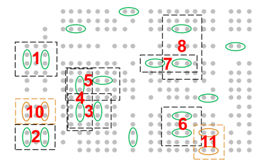
Diff-pair Crosstalk Measurement Sites

Analysis Definitions

inches2meters = 0.0254;
bd = 2e-4; % Barrel diameter, m
bdf = 1.5e-4; % Barrel finished diameter, m
ra = 3e-4; % Antipad radius, m
pr = 2.25e-4; % Pad radius, m

Frequencies of interest for the sweep:

df = 1e9;
fmax = 70e9;
freq = linspace(df,fmax,ceil(fmax/df));
Z0 = 50;

Stack Up Layer Properties

The following code defines the properties of the dielectric and metal layers. The dielectric layers are defined by dielectric objects that have different thicknesses but the same dielectric properties. The dielectric propagation constant is described as a function of frequency [3].

The metal layers are defined as metal layer objects with different thicknesses but the same copper conductor.

er = 2.8;    % Dielectric constant
tande = 0.0017; % Loss tangent
fspec = 1e9; % Frequency specification
d1 = dielectric('Name','MEG7','EpsilonR',er,'LossTangent',tande,...
    'Thickness',4.64e-3*inches2meters,'Frequency',fspec);
d2 = dielectric('Name','MEG7','EpsilonR',er,'LossTangent',tande,...
    'Thickness',4.0e-3*inches2meters,'Frequency',fspec);
d3 = dielectric('Name','MEG7','EpsilonR',er,'LossTangent',tande,...
    'Thickness',4.28e-3*inches2meters,'Frequency',fspec);
m1 = metal('Copper');
m2 = metal('Copper');
m1.Thickness = 1.200e-3*inches2meters;
m2.Thickness = 2.150e-3*inches2meters;

Test Site Signal Via Definitions

For the purpose of this example, we will limit our discussion to site 3. This section defines the location of the signal vias at the stated test site.

Signal3 = [0, -1e-3;...
    2e-3, -1e-3;...
    0, -2e-3;...
    2e-3, -2e-3];

Test Site Ground Return Via Definitions

This section defines the nearest GRVs for site 3.

Ref3 = [-1e-3 -3e-3;-1e-3 -2e-3;-1e-3 -1e-3;-1e-3 0;...
    0 -3e-3;0 0;...
    1e-3 -3e-3;1e-3 -2e-3;1e-3 -1e-3;1e-3 0;...
    2e-3 -3e-3;2e-3 0;...
    3e-3 -3e-3;3e-3 -2e-3;3e-3 -1e-3;3e-3 0];

Assemble an array of all of the GRVs.

row = cell(17,1);
row{1} = [0:4, 6, 8:13, 19];
row{2} = [-5, 1, 3, 9:15, 17:19];
row{3} = [-5, 1, 3, 9:10, 19];
row{4} = [-1:4, 6, 8:15, 18:19];
row{5} = [-5 -1 1 3 6 10 13 19];
row{6} = [-5 -1 1 3 18 19];
row{7} = [-1:4 6 10 13 19];
row{8} = [-1, 1:6, 9:13, 15, 17:19];
row{9} = [-1 1 4 10 13 19];
row{10} = [-6:-4, -2:5, 8:10, 12:15, 17:19];
row{11} = [-5 -1 1 4 10 13 19];
row{12} = -5;
row{13} = [-6:-4 -2 1 4 10 13];
row{14} = [];
row{15} = [-2 4 10 13 19];
row{16} = [-2:4, 6, 8:15, 17:19];
row{17} = [-2 1 10 13 19];

nn = 0;
for indx = 1:17
    nn = nn + size(row{indx},2);
end
RefAll = zeros(nn,2);
zndx = 0;
for indx = 1:17
    rtmp = row{indx};
    for yndx = 1:size(rtmp,2)
        RefAll(yndx+zndx,1:2) = 0.001*[rtmp(yndx),indx-7];
    end
    if ~isempty(rtmp)
        zndx = zndx+yndx;
    end
end

Site 3

The electromagnetic model used for this work is fundamentally the same as that introduced in [1]. While [1] addresses primarily single-ended vias, modeling using zero-order radial TEM waves centered on via barrels applies equally well to differential vias.

Both signal vias and ground return vias are convential through hole vias spanning from the top to the bottom of the board. The via locations, their start and stop layers are defined by a 4 column matrix. The signal via pad and signal via antipad can be defined using the antenna.Circle shape.

Define site 3 with the nearest GRVs:

start = 1;
stop = 11;
SVLocations = [Signal3 repmat([start stop],size(Signal3,1),1)];
GRVLocations = [Ref3 repmat([start stop],size(Ref3,1),1)];
vSignalViaPad = antenna.Circle('Radius',pr);

To set the single-ended (SE) ports use the 'SignalTable' property which accepts a cell array containing port information. The SE ports for each sigal via (SV) are defined at the Top (layer 1) and Bottom (layer 11).

SE Ports locations:

Port 1 - SV1 Top

Port 2 - SV2 Top

Port 3 - SV3 Top

Port 4 - SV4 Top

Port 5 - SV1 Bottom

Port 6 - SV2 Bottom

Port 7 - SV3 Bottom

Port 8 - SV4 Bottom

vPorts = {...
    1 start bd "Vertical"; ...
    2 start bd "Vertical";...
    3 start bd "Vertical";...
    4 start bd "Vertical";...
    1 stop bd "Vertical"; ...
    2 stop bd "Vertical";...
    3 stop bd "Vertical";...
    4 stop bd "Vertical"};

In the following site definition the conducting and dielectric layers of the layer stack up are defined in separate arrays, the conducting layers using metal objects and the dielectric layers using dielectric objects. The processing of this definition assumes that the metal and dielectric layers are interleaved, with the metal layers on the outside of the stack up.

The signal layers are 1, 9 and 11. The ground layers are present at 1, 3, 5, 7 and 11. For "Vertical" port connection, the start and stop layers should be defined both to be signal and ground.

obj = viaSingleEnded(...
    "SignalLayer",[start 9 stop],...
    'GroundLayer',[start:2:7 stop],...
    'Conductor',[m2 m1 m1 m1 m1 m2],...
    'Substrate',[d1 d2 d3 d2 d1],...
    'SignalViaLocations',SVLocations,...
    'SignalViaDiameter',bd,...
    "SignalViaFinishedDiameter",bdf,...
    "SignalViaPad",vSignalViaPad,...
    "RemoveUnusedPads",true,...
    'SignalViaAntipad',antenna.Circle("Radius",ra,"NumPoints",100),...
    'GroundReturnViaLocations',GRVLocations,...
    'GroundReturnViaDiameter',bd,...
    "GroundReturnViaFinishedDiameter",bdf,...
    "SignalTable",vPorts);
show(obj), view(0,90)

As shown in Figure, on Site 3 each differential port is fully surrounded by adjacent GRVs.

sparamdata = sparameters(obj,freq,Z0,"Behavioral",true);
sddmodel = s2sdd(sparamdata.Parameters,1);

s2sdd pairs the odd-numbered ports together first, followed by the even-numbered ports.

1-3 differential-mode pair 1 (SV1 Top - SV3 Top)

5-7 differential-mode pair 2 (SV1 Bottom - SV3 Bottom)

2-4 differential-mode pair 3 (SV2 Top - SV4 Top)

6-8 differential-mode pair 4 (SV2 Bottom - SV2 Bottom)

S3 = sparameters(sddmodel,sparamdata.Frequencies,2*sparamdata.Impedance);

Site 3 With All GRVs

Update site 3 with the all the GRVs from the board:

GRVLocations = [RefAll repmat([start stop],size(RefAll,1),1)];
obj.GroundReturnViaLocations = GRVLocations;
show(obj), view(0,90), zoom(2.1)

sparamdata = sparameters(obj,freq,Z0,"Behavioral",true);
sddmodel = s2sdd(sparamdata.Parameters,1);
S3_all = sparameters(sddmodel,sparamdata.Frequencies,2*sparamdata.Impedance);

You can also save the computed S-parameters as a touchstone file using syntax such as shown below:

rfwrite(S3_all,'Site3all_model.s8p','ForceOverwrite',true);

figure
title("Site 3 Near End Differential Crosstalk")
rfplot(S3,1,3)
hold on
rfplot(S3_all,1,3)
legend(["Nearest GRVs only";"All GRVs"])
legend("Location","best")

Adding all the GRVs on the test board introduces a small resonance around 50 GHz and slightly shifts the resonant peak above 60 GHz.
For site 3, having a full set of adjacent GRVs appears to come very close to fully defining the coupling between the differential ports.

The differential ports in this study have a different GRV configuration than the single-ended sites in previous studies, and the primary measurement is crosstalk rather than insertion loss.

figure
title("Site 3 modeled single-ended response")
rfplot(sparamdata,{[1 2];[1 4];[3 2];[3 4]})
legend("Location","best")

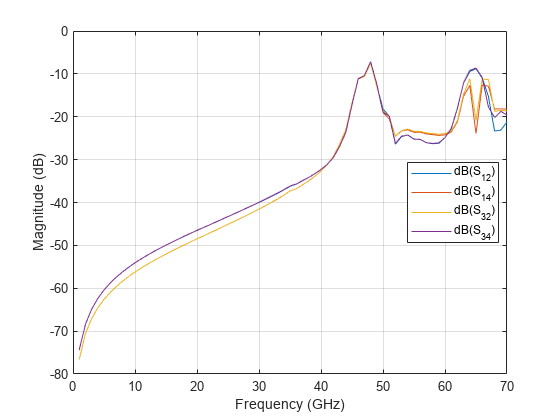
The single-ended responses S12, S14, S32 and S34 are all crosstalk coupling paths, and crosstalk coupling is the only behavior depicted in the Figure.

Summary and Conclusions

Crosstalk is carried among DSVs by waves propagating outward on ground return planes, like ripples on a pond. The presence of GRVs does not stop energy propagation, but instead simply deflects/reflects it.
At a 1 mm pitch, using GRV grids to completely surround DSVs (e.g., sites 3) provides good crosstalk isolation up to around 40 GHz. This is true regardless of the orientation of the DSVs, as per the sites mentioned.
At frequencies of interest to new interfaces standards, namely 56 to 66 GHz, computation reveals DSV crosstalk levels can rise to 20 and perhaps 10 dB, again depending on GRV configuration. Obviously, designs implementing these frequencies must pay close attention to GRV structures and choices.
Given that many physical structures exist beyond those examined herein, we recommend exploration using the mathematical models used by viaSingleEnded to adequately assess design choices.

References

Steinberger, Telian, Tsuk, Iyer and Yanamadala, “Proper Ground Return Via Placement for 40+ Gbps Signaling”, DesignCon 2022, April 2022.
Steinberger, Telian, Bell and Rowett, “Managing Differential Via Crosstalk and Ground Via Placement for 40+ Gbps Signaling”, DesignCon 2023, February 2023.
Djordjevic, Biljic, Likar-Smiljanicand and Sarkar, “Wideband Frequency-Domain Characterization of FR-4 and Time-Domain Causality”, IEEE Transactions on Electromagnetic Compatibility, Vol. 43, No. 4, pg. 662-7, November 2001.