Modeling a Family of Responses as an Uncertain System

Modeling Plant Variability as Uncertainty

In this first example, we have a family of models describing the plant behavior under various operating conditions. The nominal plant model is a first-order unstable system.

Pnom = tf(2,[1 -2])

Pnom =
 
    2
  -----
  s - 2
 
Continuous-time transfer function.

The other models are variations of Pnom. They all have a single unstable pole but the location of this pole may vary with the operating condition.

p1 = Pnom*tf(1,[.06 1]);              % extra lag
p2 = Pnom*tf([-.02 1],[.02 1]);       % time delay
p3 = Pnom*tf(50^2,[1 2*.1*50 50^2]);  % high frequency resonance
p4 = Pnom*tf(70^2,[1 2*.2*70 70^2]);  % high frequency resonance
p5 = tf(2.4,[1 -2.2]);                % pole/gain migration
p6 = tf(1.6,[1 -1.8]);                % pole/gain migration

To apply robust control tools, we can replace this set of models with a single uncertain plant model whose range of behaviors includes p1 through p6. This is one use of the command ucover. This command takes an array of LTI models Parray and a nominal model Pnom and models the difference Parray-Pnom as multiplicative uncertainty in the system dynamics.

Because ucover expects an array of models, use the stack command to gather the plant models p1 through p6 into one array.

Parray = stack(1,p1,p2,p3,p4,p5,p6);

Next, use ucover to "cover" the range of behaviors Parray with an uncertain model of the form

P = Pnom * (1 + Wt * Delta)

where all uncertainty is concentrated in the "unmodeled dynamics" Delta (a ultidyn object). Because the gain of Delta is uniformly bounded by 1 at all frequencies, a "shaping" filter Wt is used to capture how the relative amount of uncertainty varies with frequency. This filter is also referred to as the uncertainty weighting function.

Try a 4th-order filter Wt for this example:

orderWt = 4;
Parrayg = frd(Parray,logspace(-1,3,60));
[P,Info] = ucover(Parrayg,Pnom,orderWt,'InputMult');

The resulting model P is a single-input, single-output uncertain state-space (USS) object with nominal value Pnom.

P

Uncertain continuous-time state-space model with 1 outputs, 1 inputs, 5 states.
The model uncertainty consists of the following blocks:
  Parrayg_InputMultDelta: Uncertain 1x1 LTI, peak gain = 1, 1 occurrences

Type "P.NominalValue" to see the nominal value and "P.Uncertainty" to interact with the uncertain elements.

tf(P.NominalValue)

ans =
 
    2
  -----
  s - 2
 
Continuous-time transfer function.

A Bode magnitude plot confirms that the shaping filter Wt "covers" the relative variation in plant behavior. As a function of frequency, the uncertainty level is 30% at 5 rad/sec (-10dB = 0.3) , 50% at 10 rad/sec, and 100% beyond 29 rad/sec.

Wt = Info.W1;
bodemag((Pnom-Parray)/Pnom,'b--',Wt,'r'); grid
title('Relative Gaps vs. Magnitude of Wt')

You can now use the uncertain model P to design a robust controller for the original family of plant models. See Simultaneous Stabilization Using Robust Control for details.

Simplifying an Existing Uncertain Model

In this second example, we start with a detailed uncertain model of the plant. This model consists of first-order dynamics with uncertain gain and time constant, in series with a mildly underdamped resonance and significant unmodeled dynamics. This model is created using the ureal and ultidyn commands for specifying uncertain variables:

gamma = ureal('gamma',2,'Perc',30);  % uncertain gain
tau = ureal('tau',1,'Perc',30);      % uncertain time-constant
wn = 50; xi = 0.25;
P = tf(gamma,[tau 1]) * tf(wn^2,[1 2*xi*wn wn^2]);

% Add unmodeled dynamics and set SampleStateDim to 5 to get representative
% sample values of the uncertain model P.
delta = ultidyn('delta',[1 1],'SampleStateDim',5,'Bound',1);
W = makeweight(0.1,20,10);
P = P * (1+W*delta)

Uncertain continuous-time state-space model with 1 outputs, 1 inputs, 4 states.
The model uncertainty consists of the following blocks:
  delta: Uncertain 1x1 LTI, peak gain = 1, 1 occurrences
  gamma: Uncertain real, nominal = 2, variability = [-30,30]%, 1 occurrences
  tau: Uncertain real, nominal = 1, variability = [-30,30]%, 1 occurrences

Type "P.NominalValue" to see the nominal value and "P.Uncertainty" to interact with the uncertain elements.

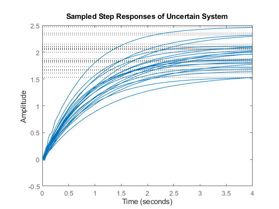
A collection of step responses illustrates the plant variability.

step(P,4)
title('Sampled Step Responses of Uncertain System')

The uncertain plant model P contains 3 uncertain elements. For control design purposes, it is often desirable to simplify this uncertainty model while approximately retaining its overall variability. This is another use of the command ucover.

To use ucover in this context, first map the uncertain model P into an array of LTI models using usample. This command samples the uncertain elements in an uncertain system and returns the corresponding LTI models, each model representing one possible behavior of the uncertain system. In this example, sample P at 60 points (the random number generator is seeded for repeatability):

rng(0,'twister');
Parray = usample(P,60);

Next, use ucover to cover all behaviors in Parray by a simple uncertainty model Usys. Choose the nominal value of P as center of the cover, and use a 2nd-order filter to model the frequency distribution of the unmodeled dynamics.

orderWt = 2;
Parrayg = frd(Parray,logspace(-3,3,60));
[Usys,Info] = ucover(Parrayg,P.NominalValue,orderWt,'InputMult');

A Bode magnitude plot shows how the filter magnitude (in red) "covers" the relative variability of the plant frequency response (in blue).

Wt = Info.W1;
bodemag((P.NominalValue-Parray)/P.NominalValue,'b--',Wt,'r')
title('Relative Gaps (blue) vs. Shaping Filter Magnitude (red)')

You can now use the simplified uncertainty model Usys to design a robust controller for the original plant, see First-Cut Robust Design for details.

Adjusting the Uncertainty Weighting

In this third example, we start with 40 frequency responses of a 2-input, 2-output system. This data has been collected with a frequency analyzer under various operating conditions. A two-state nominal model is fitted to the most typical response:

A = [-5 10;-10 -5];
B = [1 0;0 1];
C = [1 10;-10 1];
D = 0;
Pnom = ss(A,B,C,D);

The frequency response data is loaded into a 40-by-1 array of FRD models:

load ucover_demo
size(Pdata)

40x1 array of FRD models.
Each model has 2 outputs, 2 inputs, and 120 frequency points.

Plot this data and superimpose the nominal model.

bode(Pdata,'b--',Pnom,'r',{.1,1e3}), grid
legend('Frequency response data','Nominal model','Location','NorthEast')

Because the response variability is modest, try modeling this family of frequency responses using an additive uncertainty model of the form

P = Pnom + w * Delta

where Delta is a 2-by-2 ultidyn object representing the unmodeled dynamics and w is a scalar weighting function reflecting the frequency distribution of the uncertainty (variability in Pdata).

Start with a first-order filter w and compare the magnitude of w with the minimum amount of uncertainty needed at each frequency:

[P1,InfoS1] = ucover(Pdata,Pnom,1,'Additive');
w = InfoS1.W1;
bodemag(w,'r',InfoS1.W1opt,'g',{1e-1 1e3})
title('Scalar Additive Uncertainty Model')
legend('First-order w','Min. uncertainty amount','Location','SouthWest')

The magnitude of w should closely match the minimum uncertainty amount. It is clear that the first-order fit is too conservative and exceeds this minimum amount at most frequencies. Try again with a third-order filter w. For speed, reuse the data in InfoS1 to avoid recomputing the optimal uncertainty scaling at each frequency.

[P3,InfoS3] = ucover(Pnom,InfoS1,3,'Additive');
w = InfoS3.W1;
bodemag(w,'r',InfoS3.W1opt,'g',{1e-1 1e3})
title('Scalar Additive Uncertainty Model')
legend('Third-order w','Min. uncertainty amount','Location','SouthWest')

The magnitude of w now closely matches the minimum uncertainty amount. Among additive uncertainty models, P3 provides a tight cover of the behaviors in Pdata. Note that P3 has a total of 8 states (2 from the nominal part and 6 from w).

P3

Uncertain continuous-time state-space model with 2 outputs, 2 inputs, 8 states.
The model uncertainty consists of the following blocks:
  Pdata_AddDelta: Uncertain 2x2 LTI, peak gain = 1, 1 occurrences

Type "P3.NominalValue" to see the nominal value and "P3.Uncertainty" to interact with the uncertain elements.

You can refine this additive uncertainty model by using non-scalar uncertainty weighting functions, for example

P = Pnom + W1*Delta*W2

where W1 and W2 are 2-by-2 diagonal filters. In this example, restrict use W2=1 and allow both diagonal entries of W1 to be third order.

[PM,InfoM] = ucover(Pdata,Pnom,[3;3],[],'Additive');

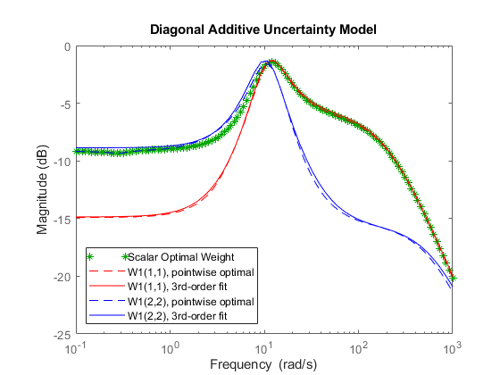
Compare the two entries of W1 with the minimum uncertainty amount computed earlier. Note that at all frequencies, one of the diagonal entries of W1 has magnitude much smaller than the scalar filter w. This suggests that the diagonally-weighted uncertainty model yields a less conservative cover of the frequency response family.

bodemag(InfoS1.W1opt,'g*',...
    InfoM.W1opt(1,1),'r--',InfoM.W1(1,1),'r',...
    InfoM.W1opt(2,2),'b--',InfoM.W1(2,2),'b',{1e-1 1e3});
title('Diagonal Additive Uncertainty Model')
legend('Scalar Optimal Weight',...
    'W1(1,1), pointwise optimal',...
    'W1(1,1), 3rd-order fit',...
    'W1(2,2), pointwise optimal',...
    'W1(2,2), 3rd-order fit',...
    'Location','SouthWest')

The degree of conservativeness of one cover over another can be partially quantified by considering the two frequency-dependent quantities:

Fd2s = norm(inv(W1)*w) ,   Fs2d = norm(W1/w)

These quantities measure by how much one uncertainty model needs to be scaled to cover the other. For example, the uncertainty model Pnom + W1*Delta needs to be enlarged by a factor Fd2s to include all of the models represented by the uncertain model Pnom + w*Delta.

Plot Fd2s and Fs2d as a function of frequency.

Fd2s = fnorm(InfoS1.W1opt*inv(InfoM.W1opt));
Fs2d = fnorm(InfoM.W1opt*inv(InfoS1.W1opt));
semilogx(fnorm(Fd2s),'b',fnorm(Fs2d),'r'), grid
axis([0.1 1000 0.5 2.6])
xlabel('Frequency (rad/s)'), ylabel('Magnitude')
title('Scale factors relating different covers')
legend('Diagonal to Scalar factor',...
    'Scalar to Diagonal factor','Location','SouthWest');

This plot shows that:

This indicates that the Pnom+W1*Delta model provides a less conservative cover of the frequency response data in Pdata.