envelope
Signal envelope
Syntax
Description
[ returns
the upper and lower envelopes of the input sequence, yupper,ylower] = envelope(x)x,
as the magnitude of its analytic signal. The analytic signal of x is
found using the discrete Fourier transform as implemented in hilbert. The function initially removes
the mean of x and adds it back after computing
the envelopes. If x is a matrix, then envelope operates
independently over each column of x.
[ returns
the envelopes of yupper,ylower] = envelope(x,fl,'analytic')x determined using the magnitude
of its analytic signal. The analytic signal is computed by filtering x with
a Hilbert FIR filter of length fl. This syntax
is used if you specify only two arguments.
[ returns
the upper and lower root-mean-square envelopes of yupper,ylower] = envelope(x,wl,'rms')x.
The envelopes are determined using a sliding window of length wl samples.
[ returns
the upper and lower peak envelopes of yupper,ylower] = envelope(x,np,'peak')x. The
envelopes are determined using spline interpolation over local maxima
separated by at least np samples.
envelope(___) with no output
arguments plots the signal and its upper and lower envelopes. This
syntax accepts any of the input arguments from previous syntaxes.
Examples
Generate a quadratic chirp modulated by a Gaussian. Specify a sample rate of 2 kHz and a signal duration of 2 seconds.
t = 0:1/2000:2-1/2000;
q = chirp(t-2,4,1/2,6,'quadratic',100,'convex').*exp(-4*(t-1).^2);
plot(t,q)
Compute the upper and lower envelopes of the chirp using the analytic signal.
[up,lo] = envelope(q);
hold on
plot(t,up,t,lo,'linewidth',1.5)
legend('q','up','lo')
hold off
The signal is asymmetric due to the nonzero mean.
Use envelope without output arguments to plot the signal and envelopes as a function of sample number.
envelope(q)
Create a two-channel signal sampled at 1 kHz for 3 seconds:
One channel is an exponentially decaying sinusoid. Specify a frequency of 7 Hz and a time constant of 2 seconds.
The other channel is a time-displaced Gaussian-modulated chirp with a DC value of 2. Specify an initial chirp frequency of 30 Hz that decays to 5 Hz after 2 seconds.
Plot the signal.
t = 0:1/1000:3;
q1 = sin(2*pi*7*t).*exp(-t/2);
q2 = chirp(t,30,2,5).*exp(-(2*t-3).^2)+2;
q = [q1;q2]';

plot(t,q)
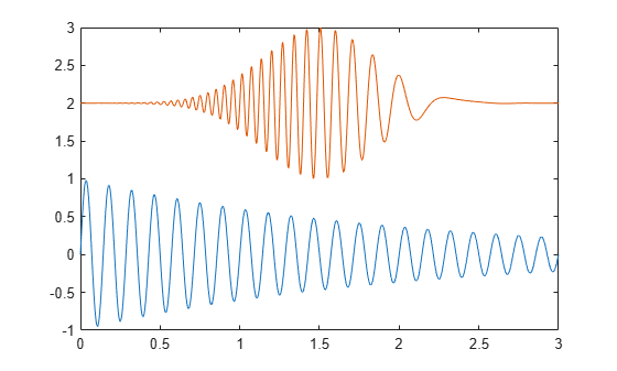
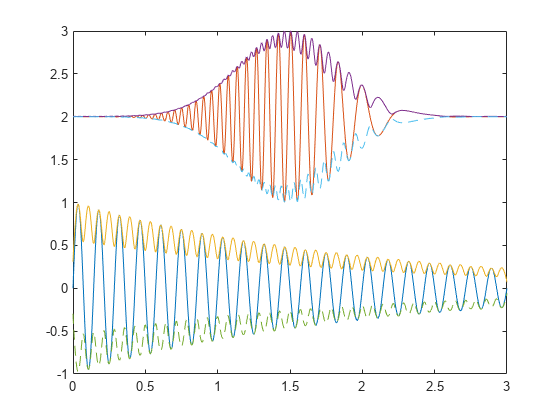
Compute the upper and lower envelopes of the signal. Use a Hilbert filter with a length of 100. Plot the channels and the envelopes. Use solid lines for the upper envelopes and dashed lines for the lower envelopes.
[up,lo] = envelope(q,100,'analytic');
hold on
plot(t,up,'-',t,lo,'--')
hold off
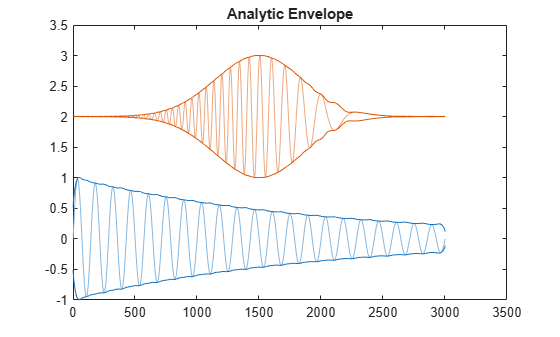
Call envelope without output arguments to produce a plot of the signal and its envelopes as a function of sample number. Increase the filter length to 300 to obtain a smoother shape. The 'analytic' flag is the default when you specify two input arguments.
envelope(q,300)
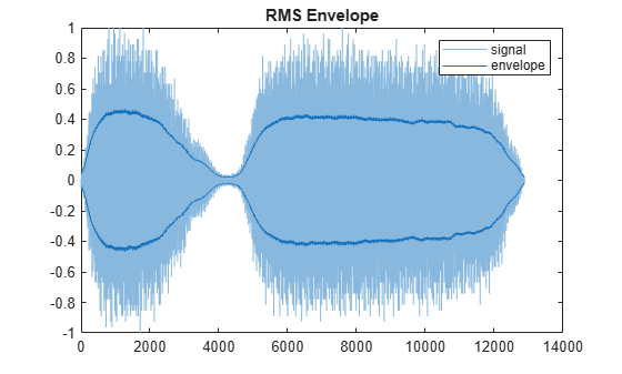
Compute and plot the moving RMS envelopes of a recording of a train whistle. Use a window with a length of 150 samples.
load('train')

envelope(y,150,'rms')
Plot the upper and lower peak envelopes of a speech signal smoothed over 30-sample intervals.
load('mtlb')

envelope(mtlb,30,'peak')
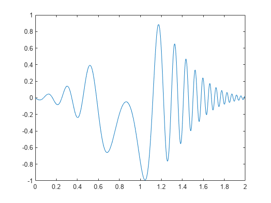
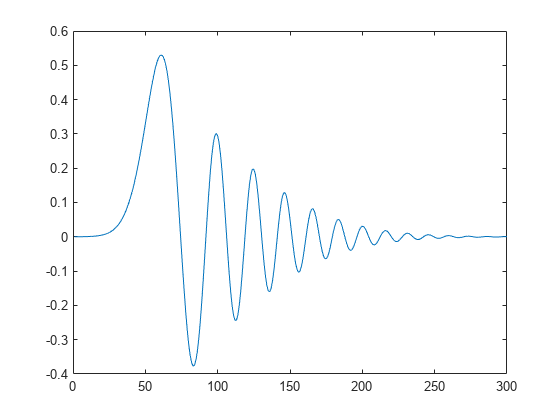
Create and plot a signal that resembles the initial detection of a light pulse propagating through a dispersive medium.
t = 0.5:-1/100:-2.49;
z = airy(t*10).*exp(-t.^2);

plot(z)
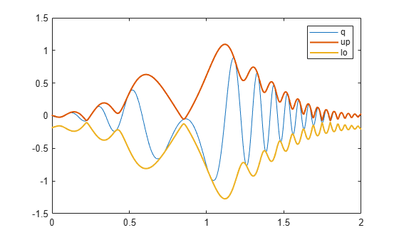
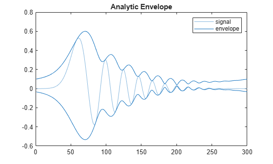
Determine the envelopes of the sequence using the magnitude of its analytic signal. Plot the envelopes.
envelope(z)
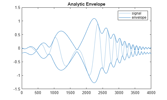
Compute the analytic envelope of the signal using a 50-tap Hilbert filter.
envelope(z,50,'analytic')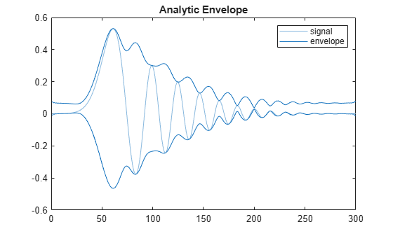
Compute the RMS envelope of the signal using a 40-sample moving window. Plot the result.
envelope(z,40,'rms')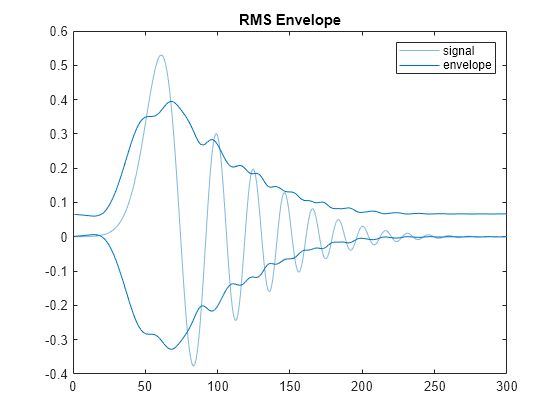
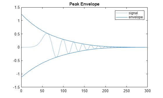
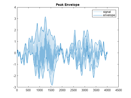
Determine the peak envelopes. Use spline interpolation with not-a-knot conditions over local maxima separated by at least 10 samples.
envelope(z,10,'peak')