idct

Inverse discrete cosine transform

Syntax

x = idct(y)

x = idct(y,n)

x = idct(y,n,dim)

y = idct(___,'Type',dcttype)

Description

x = idct(y) returns the inverse discrete cosine transform of input array y. The output x has the same size as y. If y has more than one dimension, then idct operates along the first array dimension with size greater than 1.

x = idct(y,n) zero-pads or truncates the relevant dimension of y to length n before transforming.

x = idct(y,n,dim) computes the transform along dimension dim. To input a dimension and use the default value of n, specify the second argument as empty, [].

y = idct(___,'Type',dcttype) specifies the type of inverse discrete cosine transform to compute. See Inverse Discrete Cosine Transform for details. This option can be combined with any of the previous syntaxes.

Examples

Signal Reconstruction Using Inverse Discrete Cosine Transform

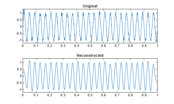
Generate a signal that consists of a 25 Hz sinusoid sampled at 1000 Hz for 1 second. The sinusoid is embedded in white Gaussian noise with variance 0.01.

rng('default')

Fs = 1000;
t = 0:1/Fs:1-1/Fs;
x = sin(2*pi*25*t) + randn(size(t))/10;

Compute the discrete cosine transform of the sequence. Determine how many of the 1000 DCT coefficients are significant. Choose 1 as the threshold for significance.

y = dct(x);

sigcoeff = abs(y) >= 1;

howmany = sum(sigcoeff)

howmany = 17

Reconstruct the signal using only the significant components.

y(~sigcoeff) = 0;

z = idct(y);

Plot the original and reconstructed signals.

subplot(2,1,1)
plot(t,x)
yl = ylim;
title('Original')

subplot(2,1,2)
plot(t,z)
ylim(yl)
title('Reconstructed')

DCT Orthogonality

Verify that the different variants of the discrete cosine transform are orthogonal, using a random signal as a benchmark.

Start by generating the signal.

s = randn(1000,1);

Verify that DCT-1 and DCT-4 are their own inverses.

dct1 = dct(s,'Type',1);
idt1 = idct(s,'Type',1);

max(abs(dct1-idt1))

ans = 1.3323e-15

dct4 = dct(s,'Type',4);
idt4 = idct(s,'Type',4);

max(abs(dct4-idt4))

ans = 1.3323e-15

Verify that DCT-2 and DCT-3 are inverses of each other.

dct2 = dct(s,'Type',2);
idt2 = idct(s,'Type',3);

max(abs(dct2-idt2))

ans = 4.4409e-16

dct3 = dct(s,'Type',3);
idt3 = idct(s,'Type',2);

max(abs(dct3-idt3))

ans = 1.1102e-15

Input Arguments

y — Input discrete cosine transform

vector | matrix | N-D array

Input discrete cosine transform, specified as a real-valued or complex-valued vector, matrix, or N-D array.

Example: dct(sin(2*pi*(0:255)/4)) specifies the discrete cosine transform of a sinusoid.

Example: dct(sin(2*pi*[0.1;0.3]*(0:39))') specifies the discrete cosine transform of a two-channel sinusoid.

Data Types: single | double
Complex Number Support: Yes

n — Inverse transform length

positive integer scalar

Inverse transform length, specified as a positive integer scalar.

Data Types: single | double

dim — Dimension to operate along

positive integer scalar

Dimension to operate along, specified as a positive integer scalar.

Data Types: single | double

dcttype — Inverse discrete cosine transform type

2 (default) | 1 | 3 | 4

Inverse discrete cosine transform type, specified as a positive integer scalar from 1 to 4.

Data Types: single | double

Output Arguments

x — Inverse discrete cosine transform

vector | matrix | N-D array

Inverse discrete cosine transform, returned as a real-valued or complex-valued vector, matrix, or N-D array.

More About

Inverse Discrete Cosine Transform

The inverse discrete cosine transform reconstructs a sequence from its discrete cosine transform (DCT) coefficients. The idct function is the inverse of the dct function.

The DCT has four standard variants. For a transformed signal y of length N, and with δ_kℓ the Kronecker delta, the inverses are defined by:

• Inverse of DCT-1:

  $$x(n)=\sqrt{\frac{2}{N-1}}{\displaystyle \sum _{k=1}^{N}y(k)\frac{1}{\sqrt{1+{\delta }_{k1}+{\delta }_{kN}}}\frac{1}{\sqrt{1+{\delta }_{n1}+{\delta }_{nN}}}\cos \left(\frac{\pi }{N-1}(k-1)(n-1)\right)}$$

• Inverse of DCT-2:

  $$x(n)=\sqrt{\frac{2}{N}}{\displaystyle \sum _{k=1}^{N}y(k)\frac{1}{\sqrt{1+{\delta }_{k1}}}\cos \left(\frac{\pi }{2N}(k-1)(2n-1)\right)}$$

• Inverse of DCT-3:

  $$x(n)=\sqrt{\frac{2}{N}}{\displaystyle \sum _{k=1}^{N}y(k)\frac{1}{\sqrt{1+{\delta }_{n1}}}\cos \left(\frac{\pi }{2N}(2k-1)(n-1)\right)}$$

• Inverse of DCT-4:

  $$x(n)=\sqrt{\frac{2}{N}}{\displaystyle \sum _{k=1}^{N}y(k)\cos \left(\frac{\pi }{4N}(2k-1)(2n-1)\right)}$$

The series are indexed from n = 1 and k = 1 instead of the usual n = 0 and k = 0, because MATLAB^® vectors run from 1 to N instead of from 0 to N – 1.

All variants of the DCT are unitary (or, equivalently, orthogonal): To find the forward transforms, switch k and n in each definition. DCT-1 and DCT-4 are their own inverses. DCT-2 and DCT-3 are inverses of each other.

References

[1] Jain, A. K. Fundamentals of Digital Image Processing. Englewood Cliffs, NJ: Prentice-Hall, 1989.

[2] Oppenheim, Alan V., Ronald W. Schafer, and John R. Buck. Discrete-Time Signal Processing. 2nd Ed. Upper Saddle River, NJ: Prentice Hall, 1999.

[3] Pennebaker, W. B., and J. L. Mitchell. JPEG Still Image Data Compression Standard. New York: Van Nostrand Reinhold, 1993.

Extended Capabilities

C/C++ Code Generation

Generate C and C++ code using MATLAB® Coder™.

Usage notes and limitations:

• C and C++ code generation for dct requires DSP System Toolbox™ software.

• The length of the transform dimension must be a power of two. If specified, the pad or truncation value must be constant. Expressions or variables are allowed if their values do not change.

• Inputs must be double precision.

GPU Arrays

Accelerate code by running on a graphics processing unit (GPU) using Parallel Computing Toolbox™.

Usage notes and limitations:

• N-D input arrays are not supported.

• The dim and dcttype input arguments are not supported.

For more information, see Run MATLAB Functions on a GPU (Parallel Computing Toolbox).

Version History

Introduced before R2006a