Battery Capacity Estimator (Least Squares, Variable Weights)
Battery capacity estimator using least-squares algorithms and variable weights
Since R2024a

Libraries:
Simscape /
Battery /
BMS /
Estimators
Description
The Battery Capacity Estimator (Least Squares, Variable Weights) block calculates the cell capacity of a battery by using least-squares algorithms. The values of the weights at the input ports VarianceSoc and VarianceCurrent can be variable.
For discrete-time simulation, set the Sample time parameter to a
positive value. To inherit the sample time, set Sample time to
-1. For continuous-time simulation, set Sample time
to 0.
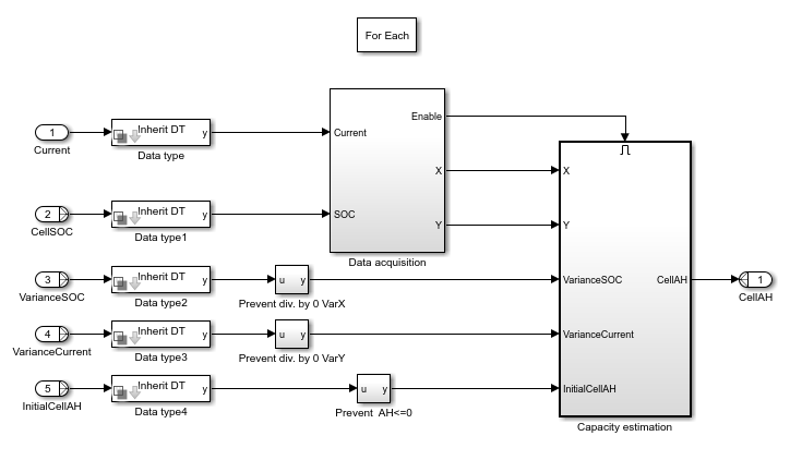
This diagram shows the structure of the block:
Equations
The least-squares estimation finds the line of best fit for a set of data points by minimizing the sum of the squared residuals. The squared residuals are the difference between the observed responses and the predicted responses of the model. This line of best fit predicts the dependent variable.
This equation defines the battery state of charge (SOC) at time tn2,
where:
SOC(tn1) is the SOC at time tn1, with n={1,…,N}.
Q is the capacity in ampere-hours.
i is the battery cell current in amperes.
denotes the integrated battery cell current over the time interval tn2 - tn1. Time tn1 and tn2 must be in hours for the units to be consistent.
Define and , and rewrite the SOC equation:
The block uses this linear equation to determine an estimate of the cell capacity using the least squares estimation,
where:
Δxn is the error associated with the SOC estimation.
Δyn is the error associated with the current sensor.
is an estimate of the true cell capacity under noisy measurements.
The weighted ordinary least squares (OLS) method estimates the cell capacity by minimizing the weighted squared errors, Δyn, of the merit function
where σ2yn denotes the variance of the current measurement and Yn is a point on the line that corresponds to the measurement data point {xn,yn}. The block assumes that yn has noise and xn has no noise.
To solve the weighted OLS problem, the block differentiates the merit function with respect to and solves for by setting the partial derivative to zero [1]:
This method can be computed recursively and is easily adapted to allow fading of past measurements.
If you define the forgetting factor as , then the block obtains the estimated capacity from the equation
where:
The weighted total least squares (TLS) method estimates the cell capacity by minimizing the sum of both weighted square errors, Δxn and Δyn, of the merit function [1],[2],
where σ2yn denotes the variance of the current measurement, σ2xn denotes the variance of the error on the SOC estimates, and Xn and Yn are points on the line that corresponds to the noisy measured data point {xn,yn}.
To enforce , the block augments the merit function with Lagrange multipliers λi:
The block sets the partial derivatives of with respect to λi, Yn, and Xn to zero:
Then the block rewrites the merit function as [1]:
Finally, the block sets the partial derivative of with respect to to zero:
In this equation:
There is no closed-form solution in the general case. To find a closed-form solution, perform a Newton-Raphson search for .
There is no recursive update in the general case.
The solution is impractical for implementation in an embedded system.
The block substitutes in the equation of :
The partial derivative of the WTLS merit function reduces to:
The block incorporates fading memory by using this equation
where:
The ATLS method is recursive and allows σ2yn and σ2xn to be non-proportional.
This figure shows the definitions the block uses to derive the approximate weighted total least squares:

The block defines Δxn and Δyn as the x-distance and y-distance between the data point n and the line, respectively. The slope of the line is for all n. The angle of the line is
This equation defines the shortest distance between the line and a given data point:
If and , the block defines the x and y components of the perpendicular distance between the data point n and the fitting line. Then the block can define the AWTLS merit function using this equation:
This equation defines the Jacobian of the AWTLS merit function:
The roots of the quartic equation are the candidate solutions for . The block rewrites the quartic equations as
where:
The ATLS merit function does not equal the weighted TLS merit function when .
When , the block uses this equation to estimate the true cell capacity:
Implementation
This figure shows how the block estimates the battery capacity using the different least-squares algorithms:

During the Data Acquisition phase, the block runs in a loop until the algorithm finds a valid data point. The block follows these steps:
The block receives an SOC estimate at time tn1 using an SOC estimator.
The block receives a second SOC estimate at time tn2.
While , the block:
Keeps receiving SOC estimates.
Integrates cell current, .
Overwrites time tn2 with a new timestamp.
If the battery is charging, the block discards the measurement and goes back to step 1.
Assumptions and Limitations
The block assumes the random errors Δxn and Δyn follow a zero-mean normal distribution.
The block assumes that the weights σ2xn and σ2yn are known.
In the RTLS algorithm, the scaling factor k must proportionally relate the weights σ2xn and σ2yn such that
Ports
Input
Output
Parameters
To edit block parameters interactively, use the Property Inspector. From the Simulink® Toolstrip, on the Simulation tab, in the Prepare gallery, select Property Inspector.
Option to specify the value of the Current input port as a vector of cell currents. If you select this parameter, the value at the Current input port can be a scalar or a vector of size equal to the size of the block inputs.
Least-square algorithm that the block uses to estimate the battery cell capacity.
Threshold to detect a change in the SOC. Typical values are 0.05 or 0.03, which represent a 5% or 3% change.
Forgetting factor.
Scaling factor k.
Dependencies
To enable this parameter, set Least squares algorithm to
Recursive total least squares or Approximate
total least squares.
Time between consecutive block executions. During execution, the block produces outputs and, if appropriate, updates its internal state. For more information, see What Is Sample Time? and Specify Sample Time.
For inherited discrete-time operation, specify this parameter as
-1. For discrete-time operation, specify this parameter as a
positive real number. For continuous-time operation, specify this parameter as
0.
If this block is in a masked subsystem or a variant subsystem that supports switching between continuous and discrete operations, promote the sample time parameter. Promoting the sample time parameter ensures correct switching between the continuous and discrete implementations of the block. For more information, see Promote Block Parameters to a Mask.
Since R2025a
Option to choose the data type for the block algorithm, specified as one of these values:
Inherit: auto— You can simulate the block in bothsingleanddoubleprecision. You must explicitly provide the inputs and parameters as eithersingleordouble.double— The block algorithm casts all inputs and parameters todoubledata type.single— The block algorithm casts all inputs and parameters tosingledata type.<data type expression>— The block algorithm casts all inputs and parameters to the data type object you specify.
Click the Show data type assistant button ![]() to display the Data Type Assistant, which helps you set the data type attributes. For more information, see Specify Data Types Using Data Type Assistant and Control Data Types of Signals.
to display the Data Type Assistant, which helps you set the data type attributes. For more information, see Specify Data Types Using Data Type Assistant and Control Data Types of Signals.
References
[1] Plett, G., Battery Management Systems: Volume II, Equivalent-Circuit Methods, Artech House, 2015.
[2] E. Bakas, B. Rosca, S. Wilkins, T. Donkers. Least-Squares-based Capacity Estimation for Lithium-ion Battery Cells, The European Battery, Hybrid and Fuel Cell Electric Vehicle Congress, Geneva, Switzerland, 2017.