SOE Estimator (Adaptive Kalman Filter, Variable Energy Capacity)

State of energy and terminal resistance estimator with Kalman filter and variable energy capacity

Since R2023b

• 

×

Libraries:
Simscape / Battery / BMS / Estimators

Description

The SOE Estimator (Adaptive Kalman Filter, Variable Energy Capacity) block implements an estimator that calculates the state of energy (SOE) and terminal resistance of a battery by using the Kalman filter algorithms. The terminal resistance, R₀, is a state of the estimator. The cell energy capacity of the battery is an input to the block.

The SOE is the ratio of the remaining energy E_remain to the total energy E_total:

$$SOE=\frac{E_{\text{remain}}}{E_{\text{total}}}.$$

This block supports single-precision and double-precision floating-point simulation.

Note

To enable single-precision floating-point simulation, the data type of all inputs and parameters, except for the Sample time (-1 for inherited) parameter, must be single.

For continuous-time simulation, set the Filter type parameter to Extended Kalman-Bucy filter or Unscented Kalman-Bucy filter.

Note

Continuous-time implementation of this block works only in a double-precision floating-point simulation. If you provide single-precision floating-point parameters and inputs, this block casts them to double-precision floating-point values to prevent errors.

For discrete-time simulation, set the Filter type parameter to Extended Kalman filter or Unscented Kalman filter and the Sample time (-1 for inherited) parameter to a positive value or -1.

Equations

These figures show the equivalent circuit for a battery with one-time-constant dynamics and two time-constant dynamics, respectively:

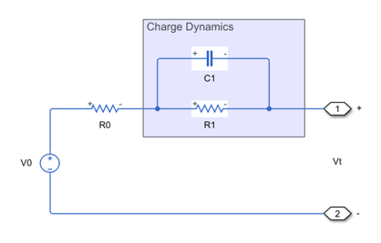
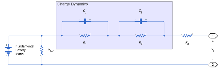
The equations for the equivalent circuit with the terminal resistance R₀ as an additional state and with two time-constant dynamics are:

$$\begin{array}{l}\frac{dSOE}{dt}=-\frac{V_{t}i}{3600E_{\text{nom}}}\\ \frac{d{V}_1}{dt}=\frac{i}{C_1\left(SOE,T\right)}-\frac{V_1}{R_1\left(SOE,T\right)C_1\left(SOE,T\right)}\\ \frac{d{V}_2}{dt}=\frac{i}{C_2\left(SOE,T\right)}-\frac{V_2}{R_2\left(SOE,T\right)C_2\left(SOE,T\right)}\\ \frac{d{R}_0}{dt}=0\\ V_{\text{t}}=V_0\left(SOE,T\right)-i{R}_0-V_1-V_2\end{array}$$

where

• SOE is the state of energy.

• i is the current.

• V₀ is the no-load voltage.

• V_t is the terminal voltage.

• E_nom is the nominal cell energy capacity.

• R₁ is the first polarization resistance.

• C₁ is the parallel RC capacitance.

• T is the temperature.

• R₀ is the terminal resistance.

• V₁ is the polarization voltage over the first RC network.

• V₂ is the polarization voltage over the second RC network.

A time constant τ₁ for the first parallel section relates the first polarization resistance R₁ and the first parallel RC capacitance C₁ using the relationship $$C_1={\tau }_1/R_1.$$

A time constant τ₂ for the second parallel section relates the second polarization resistance R₂ and the second parallel RC capacitance C₂ using the relationship $$C_2={\tau }_2/R_2.$$

For the Kalman filter algorithms, the block uses these state, input, and output vectors:

$$\begin{array}{l}x={\left[\begin{array}{ccc}SOE& V_1& R_0\end{array}\right]}^T\\ u={\left[\begin{array}{cc}{V}_{\text{t}}i& i\end{array}\right]}^T\\ y=V_{\text{t}}\end{array}$$

If you set the Charge dynamics parameter to Two time-constant dynamics, for the Kalman filter algorithms, the block uses these state, input, and output vectors:

$$\begin{array}{l}x={\left[\begin{array}{cccc}SOE& V_1& V_2& R_0\end{array}\right]}^T\\ u={\left[\begin{array}{cc}{V}_{\text{t}}i& i\end{array}\right]}^T\\ y=V_{\text{t}}\end{array}$$

Then the block rewrites the equations for the equivalent circuit as a standard nonlinear state space system:

$$\begin{array}{l}\dot{x}=f\left(x,u\right)\\ y=h\left(x,u\right)\end{array}$$

The linearized model is

$$\begin{array}{l}\delta \dot{x}=A\left(k\right)\delta x+B\left(k\right)\delta u\\ \delta y=C\left(k\right)\delta x+D\left(k\right)\delta u\end{array}$$

where:

$$\begin{array}{l}A\left(k\right)=\frac{\delta f\left(x,u\right)}{\delta x}\\ B\left(k\right)=\frac{\delta f\left(x,u\right)}{\delta u}\\ C\left(k\right)=\frac{\delta h\left(x,u\right)}{\delta x}\\ D\left(k\right)=\frac{\delta h\left(x,u\right)}{\delta u}\end{array}$$

Extended Kalman Filter

This diagram shows the structure of the extended Kalman filter (EKF):

For a battery SOE estimation technique with a one-time-constant model, the block uses this linearized model:

$$\begin{array}{l}{A}_d\left(k\right)=\left[\begin{array}{ccc}1& 0& 0\\ 0& e^{\frac{-T_{\text{s}}}{R_1{C}_1}}& 0\\ 0& 0& 1\end{array}\right]\\ B_d\left(k\right)=\left[\begin{array}{cc}-\frac{T_{\text{s}}}{3600E_{\text{nom}}}& 0\\ 0& R_1\left(1-e^{\frac{-T_{\text{s}}}{R_1{C}_1}}\right)\\ 0& 0\end{array}\right]\\ C_d\left(k\right)=\left[\begin{array}{ccc}\frac{\delta V_{\text{OC}}}{\delta SOE}& \frac{\delta V}{\delta V_1}& \frac{\delta V}{\delta R_0}\end{array}\right]=\left[\begin{array}{ccc}\frac{\delta V_{\text{OC}}}{\delta SOE}& -1& -i\end{array}\right]\end{array}$$

You can modify three parameters of the Kalman filter: the covariance of the measurement noise R, the initial state error covariance P₀, and the covariance of the process noise Q. Set R to the square of the error from the equipment you used to test the battery cell.

The EKF algorithm comprises these phases:

• Initialization

  • $$\widehat{x}(0|0)$$⁠— State estimate at time step 0 using measurements at time step 0.

  • $$\widehat{P}(0|0)$$⁠— State estimation error covariance matrix at time step 0 using measurements at time step 0.

• Prediction

  • Project the states ahead (a priori):

    $$\widehat{x}\left(k+1|k\right)=A_d\left(k\right)\widehat{x}\left(k|k\right)+B_d\left(k\right)u\left(k\right)$$

  • Project the error covariance ahead:

    $$\widehat{P}\left(k+1|k\right)=A_d\left(k\right)\widehat{P}\left(k|k\right)A_d^T\left(k\right)+Q,$$

    where Q is the covariance of the process noise.

• Correction

  • Compute the Kalman gain:

    $$K(k+1)=\widehat{P}(k+1|k)C_d^T(k){(C_d(k)\widehat{P}(k+1|k)C_d^T(k)+R)}^{-1},$$

    where R is the covariance of the measurement noise.

  • Update the estimate with the measurement y(k) (a posteriori):

    $$\widehat{x}\left(k+1|k+1\right)=\widehat{x}\left(k+1|k\right)+K\left(k+1\right)\left(y\left(k\right)-C_d\widehat{x}\left(k+1|k\right)\right).$$

  • Update the error covariance:

    $$\widehat{P}\left(k+1|k+1\right)=\left(1-K\left(k+1\right)C_d\right)\widehat{P}\left(k+1|k\right).$$

Extended Kalman-Bucy Filter

This diagram shows the structure of the extended Kalman-Bucy filter (EKBF):

The EKBF is the continuous-time variant of the Kalman filter.

$$\begin{array}{l}\frac{dx\left(t\right)}{dt}=f\left(x\left(t\right),u\left(t\right)\right)+w\left(t\right)\\ y\left(t\right)=h\left(x\left(t\right),u\left(t\right)\right)+v\left(t\right)\end{array}$$

In continuous time, the EKBF couples the prediction and correction steps.

• Initialization

  • $$\widehat{x}(t_0)=E\left[x\left(t_0\right)\right]$$⁠— State estimate at time t₀.

  • $$\widehat{P}(t_0)=\mathrm{var}\left[x\left(t_0\right)\right]$$⁠— State estimation error covariance matrix at time t₀.

• Prediction-Correction EKBF algorithm

  $$\begin{array}{l}K\left(t\right)=P\left(t\right)H^T\left(t\right)R^{-1}\left(t\right)\\ \frac{d\widehat{x}\left(t\right)}{dt}=f\left(\widehat{x}\left(t\right),u\left(t\right)\right)+K\left(t\right)\left(y\left(t\right)-h\left(\widehat{x}\left(t\right),u\left(t\right)\right)\right)\\ \frac{dP\left(t\right)}{dt}=F\left(t\right)P\left(t\right)+P\left(t\right)F^T\left(t\right)+Q\left(t\right)-K\left(t\right)H\left(t\right)P\left(t\right)\end{array}$$

  where:

  $$\begin{array}{l}F\left(t\right)=\frac{\partial f}{\partial x}\\ H\left(t\right)=\frac{\partial h}{\partial x}\end{array}$$

Unscented Kalman Filter

This diagram shows the structure of the unscented Kalman filter (UKF):

The EKF locally approximates nonlinear functions with the linear equations obtained from the Taylor expansion by using only the first term of the expansion. In a highly nonlinear system, these solutions are not very accurate.

The UKF uses nonlinear transformations on a set of sigma points that the algorithm chooses deterministically. This technique is called unscented transformation. The mean and the covariance matrix of the transformed points are accurate to the second order of the Taylor series expansion.

The algorithm first generates a set of state values called sigma points. These sigma points capture the mean and covariance of the state estimates. The algorithm uses each of the sigma points as an input to the state transition and measurement functions to get a new set of transformed state points. Then, the algorithm uses the mean and covariance of the transformed points to obtain state estimates and state estimation error covariance.

The UKF algorithm follows these steps:

• Initialization

  • $$\widehat{x}(0|0)=E\left[x\left(0\right)\right]$$⁠— State estimate at time step 0 using measurements at time step 0.

  • $$\widehat{P}(0|0)=P\left(0\right)$$⁠— State estimation error covariance matrix at time step 0 using measurements at time step 0.

• Generate sigma points and calculate the mean weight and covariance weight for each point.

  • Choose the sigma points x⁽ⁱ⁾(k|k)

    $$\begin{array}{l}{x}^{(i)}\left(k|k\right)=\{\begin{array}{cc}\widehat{x}\left(k+1|k\right)& i=1\\ \widehat{x}\left(k+1|k\right)+{\left(\sqrt{\left(n+\lambda \right)P\left(k|k\right)}\right)}_i& i=2,\dots ,n+1\\ \widehat{x}\left(k+1|k\right)-{\left(\sqrt{\left(n+\lambda \right)P\left(k|k\right)}\right)}_i& i=n+2,\dots ,2n+1\end{array}\\ W_m^{(i)}=\{\begin{array}{cc}\frac{\lambda }{n+\lambda }& i=1\\ \frac{1}{2\left(n+\lambda \right)}& i\ne 1\end{array}\\ W_c^{(i)}=\{\begin{array}{cc}\frac{\lambda }{n+\lambda }+\left(1-{\alpha }^2+\beta \right)& i=1\\ \frac{1}{2\left(n+\lambda \right)}& i\ne 1\end{array}\end{array}$$

    where:

    • n is the dimension of the state vector, x.

    • $$\lambda ={\alpha }^2\left(n+\kappa \right)-n,\alpha \in \left[0,1\right]$$ describes the distance between the sigma point and the mean point. In a normal distribution, β = 2 and κ = 0.

    • $${\left(\sqrt{\left(n+\lambda \right)P}\right)}_i$$ is the ith row or column of $$\sqrt{cP}$$. The block calculates the matrix square root by using numerically efficient and stable methods such as the Cholesky decomposition.

• Perform first estimation of the system state matrix:

  $$\begin{array}{l}{\widehat{x}}^{(i)}\left(k+1|k\right)=f\left({\widehat{x}}^{(i)}\left(k|k\right),u\left(k\right)\right)\\ \widehat{x}\left(k+1|k\right)={\displaystyle \sum _{i=1}^{2n+1}{W}_m^{\left(i\right)}}{\widehat{x}}^{\left(i\right)}\left(k+1|k\right)\end{array}$$

• Perform first estimation of the covariance matrix of the state variables:

  $$P\left(k+1|k\right)={\displaystyle \sum _{i=1}^{2n+1}{W}_c^{(i)}\left({\widehat{x}}^{(i)}\left(k+1|k\right)-\widehat{x}\left(k+1|k\right)\right)\cdot {\left({\widehat{x}}^{(i)}\left(k+1|k\right)-\widehat{x}\left(k+1|k\right)\right)}^T}+Q$$

• Estimate the measured variables:

  $$\begin{array}{l}{y}^{\left(i\right)}\left(k+1|k\right)=h\left({\widehat{x}}^{(i)}\left(k+1|k\right),u\left(k\right)\right)\\ \widehat{y}\left(k+1|k\right)={\displaystyle \sum _{i=1}^{2n+1}{W}_m^{(i)}{\widehat{y}}^{\left(i\right)}\left(k+1|k\right)}\end{array}$$

• Estimate the covariance of the measurement (P_y) and covariance between the measurement and the state (P_xy):

  $$\begin{array}{l}{P}_y={\displaystyle \sum _{i=1}^{2n+1}{W}_c^{\left(i\right)}\left({\widehat{y}}^{\left(i\right)}\left(k+1|k\right)-\widehat{y}\left(k+1|k\right)\right)\cdot {\left({\widehat{y}}^{\left(i\right)}\left(k+1|k\right)-\widehat{y}\left(k+1|k\right)\right)}^T+R}\\ P_{xy}={\displaystyle \sum _{i=1}^{2n+1}\left({\widehat{x}}^{\left(i\right)}\left(k+1|k\right)-\widehat{x}\left(k+1|k\right)\right)\cdot {\left({\widehat{y}}^{\left(i\right)}\left(k+1|k\right)-\widehat{y}\left(k+1|k\right)\right)}^T}\end{array}$$

• Compute the Kalman filter gain:

  $$K\left(k+1\right)=P_{xy}{P}_y^{-1}$$

• Perform the second update of the state matrix and of the covariance of the state variables:

  $$\begin{array}{l}\widehat{x}\left(k+1|k+1\right)=\widehat{x}\left(k+1|k\right)+K\left(k+1\right)\left(y\left(k+1\right)-\widehat{y}\left(k+1|k\right)\right)\\ P\left(k+1|k+1\right)=P\left(k+1|k\right)-K\left(k+1\right)P_y{K}^T\left(k+1\right)\end{array}$$

Unscented Kalman-Bucy Filter

This diagram illustrates the overall structure of the unscented Kalman-Bucy filter (UKBF):

The derived continuous-time filtering equations of the UKBF are similar to the EKBF equations.

The stochastic differential equations corresponding to the UKF in continuous time are:

$$\begin{array}{l}K\left(t\right)=X\left(t\right)W{h}^T\left(X(t),t\right)R^{-1}(t)\\ \frac{dm\left(t\right)}{dt}=f\left(X\left(t\right),t\right)w_m+K\left(t\right)\left(y\left(t\right)-h\left(X\left(t\right),t\right)w_m\right)\\ \frac{dP\left(t\right)}{dt}=X\left(t\right)W{f}^T\left(X\left(t\right),t\right)+f\left(X\left(t\right),t\right)W{X}^T\left(t\right)+Q\left(t\right)-K\left(t\right)R\left(t\right)K^T\left(t\right)\end{array}$$

where

• $$X\left(t\right)=\left[\begin{array}{ccc}m\left(t\right)& \dots & m\left(t\right)\end{array}\right]+\sqrt{c}\left[\begin{array}{ccc}0& \sqrt{P\left(t\right)}& -\sqrt{P\left(t\right)}\end{array}\right]$$ is the sigma-point matrix.

• $$w_m={\left[\begin{array}{ccc}{W}_m^{\left(1\right)}& \cdots & W_m^{\left(2n+1\right)}\end{array}\right]}^T$$

• $$W=\left(I-\left[\begin{array}{ccc}{w}_m& \cdots & w_m\end{array}\right]\right)\text{diag}\left(\begin{array}{ccc}{W}_c^{\left(1\right)}& \cdots & W_c^{\left(2n+1\right)}\end{array}\right){\left(I-\left[\begin{array}{ccc}{w}_m& \cdots & w_m\end{array}\right]\right)}^T$$

• $$c={\alpha }^2\left(n+\kappa \right)$$

The general UKBF equations can run into issues related to finite numerical precision of computer arithmetic. Because the UKF uses matrix square roots in its sigma points, the square-root UKBF algorithm obtains the square-root version of the UKBF by formulating the filter as a differential equation for the sigma points. The equations for the square-root UKBF are:

$$\begin{array}{l}K\left(t\right)=X\left(t\right)W{h}^T\left(X(t),t\right)R^{-1}(t)\\ M\left(t\right)=A^{-1}\left(t\right)\left[X\left(t\right)W{f}^T\left(X\left(t\right),t\right)+f\left(X\left(t\right),t\right)W{X}^T\left(t\right)+Q\left(t\right)-K\left(t\right)R\left(t\right)K^T\left(t\right)\right]A^{-T}\left(t\right)\\ \frac{d{X}_i\left(t\right)}{dt}=f\left(X\left(t\right),t\right)w_m+K\left(t\right)\left(y\left(t\right)-h\left(X\left(t\right),t\right)w_m\right)+\sqrt{c}{\left[\begin{array}{ccc}0& A\left(t\right)\Phi \left(M\left(t\right)\right)& -A\left(t\right)\Phi \left(M\left(t\right)\right)\end{array}\right]}_i\end{array}$$

where

• $$X\left(t\right)=\left[\begin{array}{ccc}m\left(t\right)& \dots & m\left(t\right)\end{array}\right]+\sqrt{c}\left[\begin{array}{ccc}0& A\left(t\right)& -A\left(t\right)\end{array}\right]$$ is the sigma-point matrix.

• $${\Phi }_{ij}\left(M\left(t\right)\right)=\{\begin{array}{cc}{M}_{ij}\left(t\right),& i>j\\ 0.5M_{ij}\left(t\right),& i=j\\ 0,& i<j\end{array}$$ is a function that returns the lower diagonal part of the argument.

• $${\left[\begin{array}{ccc}0& A\left(t\right)\Phi \left(M\left(t\right)\right)& -A\left(t\right)\Phi \left(M\left(t\right)\right)\end{array}\right]}_i$$ is the ith column of the argument matrix.

This matrix implementation is not always the most computationally efficient implementation of the square-root UKBF. You can use these equations to alternatively compute the matrix expressions:

$$\begin{array}{l}X\left(t\right)W{f}^T\left(X\left(t\right),t\right)={\displaystyle \sum _{i=1}^{2n+1}{W}_c^{\left(i\right)}\left(x^{\left(i\right)}-m_x\right){\left(f\left(x^{\left(i\right)},t\right)-m_f\right)}^T}\\ f\left(X\left(t\right),t\right)W{X}^T\left(t\right)={\displaystyle \sum _{i=1}^{2n+1}{W}_c^{\left(i\right)}\left(f\left(x^{\left(i\right)},t\right)-m_f\right){\left(x^{\left(i\right)}-m_x\right)}^T}\\ X\left(t\right)W{h}^T\left(X\left(t\right),t\right)={\displaystyle \sum _{i=1}^{2n+1}{W}_c^{\left(i\right)}\left(x^{\left(i\right)}-m_x\right){\left(h\left(x^{\left(i\right)},t\right)-m_h\right)}^T}\end{array}$$

where

$$\begin{array}{l}{m}_x={\displaystyle \sum _{i=1}^{2n+1}{W}_m^{\left(i\right)}{x}^{\left(i\right)}}\\ m_f={\displaystyle \sum _{i=1}^{2n+1}{W}_m^{\left(i\right)}f\left(x^{\left(i\right)},t\right)}\\ m_h={\displaystyle \sum _{i=1}^{2n+1}{W}_m^{\left(i\right)}h\left(x^{\left(i\right)},t\right)}\end{array}$$

Ports

Input

Current — Battery current, ampere

scalar | vector

Battery current, in ampere, specified as a scalar for a single cell or a vector for multiple cells. To specify this input as a vector of cell currents, select the Specify Current input as cell current(s) parameter.

CellVoltage — Cell voltage, volt

scalar | vector

Cell voltage, in volt, specified as a scalar for a single cell or a vector for multiple cells. The size of this input port must be equal to the size of the CellTemperature, EnergyCapacity, InitialSOE, and InitialR0 input ports.

CellTemperature — Cell temperature, celsius or kelvin

scalar | vector

Cell temperature, specified as a scalar for a single cell or a vector for multiple cells. The size of this input port must be equal to the size of the CellVoltage, EnergyCapacity, InitialSOE, and InitialR0 input ports.

EnergyCapacity — Cell energy capacity, W*Hr

scalar | vector

Cell energy capacity of the battery, in watt-hour, specified as a scalar for a single cell or a vector for multiple cells. The block calculates the state of charge by dividing the accumulated charge by this value. The block calculates the accumulated charge by integrating the battery current.

The size of this input port must be equal to the size of the CellTemperature, CellVoltage, InitialSOE, and InitialR0 input ports.

InitialSOE — Initial state of energy, unitless

scalar | vector

Initial state of energy, specified as a scalar or vector of entries in the range [0, 1]. The size of this input port must be equal to the size of the CellVoltage, CellTemperature, EnergyCapacity, and InitialR0 input ports.

InitialR0 — Initial terminal resistance, ohm

scalar | vector

Initial terminal resistance, specified as a scalar or a vector. The size of this input port must be equal to the size of the CellVoltage, CellTemperature, EnergyCapacity, and InitialSOE input ports.

Output

SOE — State of energy, unitless

scalar | vector

State of energy of the battery, returned as a scalar or a vector. The size of this output port is equal to the size of the CellVoltage, CellTemperature, EnergyCapacity, InitialSOE, and InitialR0 input ports.

Parameters

Main

Specify Current input as cell current(s) — Option to specify current input port as vector

off (default) | on

Option to specify the value of the Current input port as a vector of cell currents. If you select this parameter, the value at the Current input port can be a scalar or a vector of size equal to the size of the block inputs.

Filter type — Kalman filter type

Extended Kalman filter (default) | Extended Kalman-Bucy filter | Unscented Kalman filter | Unscented Kalman-Bucy filter

Type of Kalman filter that this block uses to estimate the state of energy of the battery.

Alpha — Alpha coefficient

1 (default) | scalar in the range [0, 1]

Coefficient that controls the spread of the sigma points. The block uses this parameter in its implementation of the equations for the unscented Kalman filter and the unscented Kalman-Bucy filter.

Dependencies

To enable this parameter, set Filter type to Unscented Kalman filter or Unscented Kalman-Bucy filter.

Beta — Beta coefficient

2 (default) | nonnegative scalar

Coefficient related to the distribution. The block uses this parameter in its implementation of the unscented Kalman filter and the unscented Kalman-Bucy filter.

Dependencies

To enable this parameter, set Filter type to Unscented Kalman filter or Unscented Kalman-Bucy filter.

Kappa — Kappa coefficient

0 (default) | scalar in the range [0, 3]

Coefficient that controls the spread of the sigma points. The block uses this parameter in its implementation of the equations for the unscented Kalman filter and the unscented Kalman-Bucy filter.

Dependencies

To enable this parameter, set Filter type to Unscented Kalman filter or Unscented Kalman-Bucy filter.

Covariance of the process noise, Q — Covariance of the process noise

[1e-6 0 0; 0 1e-6 0;0 0 1e-6] (default) | matrix of scalars

3-by-3 covariance matrix of the noise in the states.

Covariance of the measurement noise, R — Covariance of the measurement noise

0.1 (default) | scalar

Covariance of the noise in the measurements.

Initial state error covariance, P0 — Initial state error covariance

[1e-5 0 0; 0 1 0; 0 0 1e-5] (default) | matrix of scalars

3-by-3 covariance matrix of the initial state error. This parameter defines the deviation in the initialization of the state.

Sample time (-1 for inherited) — Block sample time

1 (default) | 0 | -1 | integer

Time between consecutive block executions. During execution, the block produces outputs and, if appropriate, updates its internal state. For more information, see What Is Sample Time? and Specify Sample Time.

For inherited discrete-time operation, specify this parameter as -1. For discrete-time operation, specify this parameter as a positive integer. For continuous-time operation, specify this parameter as 0.

If this block is in a masked subsystem or a variant subsystem that supports switching between continuous operation and discrete operation, promote the sample time parameter. Promoting the sample time parameter ensures correct switching between the continuous and discrete implementations of the block. For more information, see Promote Block Parameters on a Mask.

Dependencies

To enable this parameter, set Filter type to Extended Kalman filter or Unscented Kalman filter.

System Model

Charge dynamics — Option to model battery charge dynamics

One time-constant dynamics (default) | Two time-constant dynamics

Since R2024a

Option to model the battery charge dynamics. This parameter determines the number of parallel RC sections in the equivalent circuit:

• One time-constant dynamics — The equivalent circuit contains one parallel RC section. Specify the polarization resistance and the time constant using the First polarization resistance, R1(SOE,T), (ohm) and First time constant, tau1(SOE,T), (s) parameters.

• Two time-constant dynamics — The equivalent circuit contains two parallel RC sections. Specify the polarization resistances and the time constants using the First polarization resistance, R1(SOE,T), (ohm), First time constant, tau1(SOE,T), (s), Second polarization resistance, R2(SOE,T), (ohm), and Second time constant, tau2(SOE,T), (s) parameters.

Vector of state-of-energy values, SOE (-) — SOE breakpoints

[0, .1, .25, .5, .75, .9, 1] (default) | vector of scalars in the range [0, 1]

Vector of the SOE breakpoints defining the points at which you specify lookup data. The entries of this vector must be in strictly ascending order. The block calculates the SOE value with respect to the nominal battery energy capacity specified at the EnergyCapacity port.

Vector of temperatures, T — Temperature breakpoints

[278, 293, 313] (default) | vector of positive scalars

Vector of temperature breakpoints defining the points at which you specify lookup data. This vector must be strictly ascending and greater than 0 K. The physical unit of this parameter must be the same as the physical unit of the CellTemperature input port.

First polarization resistance, R1(SOE,T), (ohm) — First RC resistance at temperature breakpoints

[.0109, .0029, .0013; .0069, .0024, .0012; .0047, .0026, .0013; .0034, .0016, .001; .0033, .0023, .0014; .0033, .0018, .0011; .0028, .0017, .0011] (default) | matrix of positive entries

Lookup data, in ohm, for the first parallel RC resistance at the specified SOE and temperature breakpoints. The number of rows of this matrix is equal to the size of the Vector of state-of-energy values, SOE (-) parameter. The number of columns of this matrix is equal to the size of the Vector of temperatures, T parameter.

First time constant, tau1(SOE,T), (s) — First RC time constant at temperature breakpoints

[20, 36, 39; 31, 45, 39; 109, 105, 61; 36, 29, 26; 59, 77, 67; 40, 33, 29; 25, 39, 33] (default) | matrix of positive entries

Lookup data, in seconds, for the first parallel RC time constant at the specified SOE and temperature breakpoints. The number of rows of this matrix is equal to the size of the Vector of state-of-energy values, SOE (-) parameter. The number of columns of this matrix is equal to the size of the Vector of temperatures, T parameter.

Second polarization resistance, R2(SOE,T), (ohm) — Second RC resistance at temperature breakpoints

[.0109, .0029, .0013; .0069, .0024, .0012; .0047, .0026, .0013; .0034, .0016, .001; .0033, .0023, .0014; .0033, .0018, .0011; .0028, .0017, .0011] (default) | matrix of positive entries

Since R2024a

Lookup data, in ohm, for the Second parallel RC resistance at the specified SOE and temperature breakpoints. The number of rows of this matrix is equal to the size of the Vector of state-of-energy values, SOE (-) parameter. The number of columns of this matrix is equal to the size of the Vector of temperatures, T parameter.

Dependencies

To enable this parameter, set Charge dynamics to Two time-constant dynamics.

Second time constant, tau2(SOE,T), (s) — Second RC time constant at temperature breakpoints

[20, 36, 39; 31, 45, 39; 109, 105, 61; 36, 29, 26; 59, 77, 67; 40, 33, 29; 25, 39, 33] (default) | matrix of positive scalars

Since R2024a

Lookup data, in seconds, for the Second parallel RC time constant at the specified SOE and temperature breakpoints. The number of rows of this matrix is equal to the size of the Vector of state-of-energy values, SOE (-) parameter. The number of columns of this matrix is equal to the size of the Vector of temperatures, T parameter.

Dependencies

To enable this parameter, set Charge dynamics to Two time-constant dynamics.

No-load voltage, V0(SOE,T), (V) — V₀ lookup table

[3.49, 3.5, 3.51; 3.55, 3.57, 3.56; 3.62, 3.63, 3.64; 3.71, 3.71, 3.72; 3.91, 3.93, 3.94; 4.07, 4.08, 4.08; 4.19, 4.19, 4.19] (default) | matrix of nonnegative entries

Lookup data, in volt, for open-circuit voltages across the fundamental battery model at the specified SOE. The number of rows of this matrix is equal to the size of the Vector of state-of-energy values, SOE (-) parameter. The number of columns of this matrix is equal to the size of the Vector of temperatures, T parameter.

References

[1] Yujie Wang, Chenbin Zhang, Zonghai Chen. Model-based State-of-energy Estimation of Lithium-ion Batteries in Electric Vehicles. Energy Procedia, Volume 88, 2016, Pages 998-1004.

[2] S. Munisamy, D. J. Auger, A. Fotouhi, B. Hawkes and E. Kappos, State of energy estimation in electric propulsion systems with lithium-sulfur batteries. Online Conference, 2020, pp. 788-795.

[3] R. Van der Merwe and E. A. Wan, The square-root unscented Kalman filter for state and parameter-estimation. 2001 IEEE International Conference on Acoustics, Speech, and Signal Processing. Proceedings (Cat. No.01CH37221), 2001, pp. 3461-3464 vol.6, doi: 10.1109/ICASSP.2001.940586.

[4] M. S. Grewal and A. P. Andrews, Kalman Filtering, Theory and Practice Using MATLAB. New York: Wiley Intersci., 2001.

[5] S. Sarkka, On Unscented Kalman Filtering for State Estimation of Continuous-Time Nonlinear Systems. IEEE Transactions on Automatic Control, vol. 52, no. 9, pp. 1631-1641, Sept. 2007, doi: 10.1109/TAC.2007.904453.

Extended Capabilities

C/C++ Code Generation
Generate C and C++ code using Simulink® Coder™.

Version History

Introduced in R2023b

R2024a: Estimate SOE using equivalent models with two time-constant charge dynamics

You can now estimate the battery SOE by using equivalent models with two time-constant charge dynamics.

To select an equivalent model with two time-constant charge dynamics, set the Charge dynamics parameter to Two time-constant dynamics and specify the values of the new Second polarization resistance, R2(SOE,T), (ohm) and Second time constant, tau2(SOE,T), (s) parameters.