Run Parameter Sweep in Rapid Accelerator Mode Using Parallel Simulations

This example shows how to run multiple accelerated simulations in parallel by using parsim and Parallel Computing Toolbox™. Run Parameter Sweep Using Parallel Simulations shows how to use multiple cores of your host machine to run independent simulations while varying a parameter. In this example, use rapid accelerator mode to speed up multiple simulations even further. If you do not have Parallel Computing Toolbox or MATLAB Parallel Server™, the simulations in this example run serially.

Explore Model

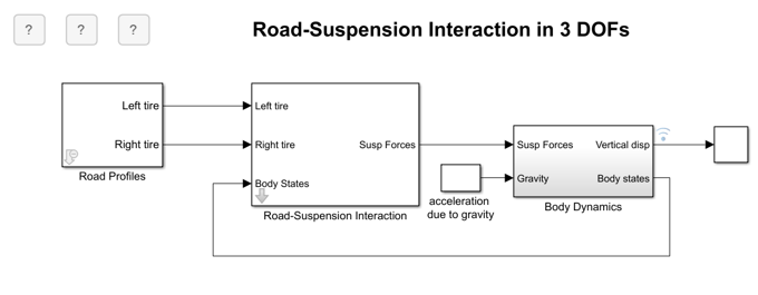
This example uses the same model as the example Run Parameter Sweep Using Parallel Simulations. The model sldemo_suspn_3dof simulates vehicle dynamics based on the interaction between road and suspension for different road profiles. In this Monte Carlo study, vary the vehicle mass to study its effect on the vehicle dynamics. The example uses rapid accelerator mode simulation and Parallel Computing Toolbox to speed up these multiple simulations.

mdl = "sldemo_suspn_3dof";
open_system(mdl);

To log the vertical vehicle displacement over time, the signal connected to the Vertical disp output port of the Body Dynamics subsystem is marked for signal logging, as indicated by the logging badge. To examine the logging settings, right-click the signal and select Properties. In the Signal Properties dialog box, the Log signal data parameter is selected and the signal is configured to log data using the custom logging name vertical_disp.

Prepare Parameter Inputs

Calculate the sweep values for the vehicle mass as factors of the design value ranging from 0.5 to 9.5 in increments of 1. Store the sweep values in a variable, Mb_sweep, in the base workspace.

Mb_sweep = Mb*(0.5:1:9.5);

The number of simulations to run is equal to the number of sweep values. Store the number in a variable, numSims.

numSims = length(Mb_sweep);

Use vectorization and a for loop to:

1. Preallocate an array of Simulink.SimulationInput objects for the model, one per simulation, and store them in the variable in.

2. Set model parameters for all simulations at once using setModelParameter function on the array of SimulationInput objects. In particular, configure the model for rapid accelerator mode simulation. Set RapidAcceleratorUpToDateCheck to off because the model structure does not change between simulations, allowing reuse of the build files.

3. Specify simulation-specific values for each SimulationInput object using the setVariable function.

Specifying the model parameter on the SimulationInput object applies it to the model only during the simulation. The software applies the specified value during simulation and reverts to the original value, if possible, after the simulation finishes.

in(1:numSims) = Simulink.SimulationInput(mdl);

in = in.setModelParameter("SimulationMode","rapid-accelerator", ...
    "RapidAcceleratorUpToDateCheck","off");
for i = 1:numSims
    in(i) = in(i).setVariable("Mb",Mb_sweep(i));
end

Build Rapid Accelerator Target

parsim provides a SetupFcn option to specify a function to run once per worker before starting simulations. Write a function for this option that builds the simulation target. The simulation target is built once and used by all subsequent simulations, reducing the time required for model compilation. In the function, change the current folder on the workers to an empty folder so that any existing slprj folder on the client does not interfere with the build process.

function build_rapid_accel_if_required(mdl, clientArch)
    workerArch = computer("arch");
    if ~strcmp(clientArch,workerArch)
        currentFolder = pwd;
        tempDir = tempname;
        mkdir(tempDir);
        cd (tempDir);
        oc = onCleanup(@() cd (currentFolder));
        Simulink.BlockDiagram.buildRapidAcceleratorTarget(mdl);
    end
end

Run Simulations in Parallel

To execute the simulations in parallel, use parsim on the array of SimulationInput objects. The parsim command returns an array of Simulink.SimulationOutput objects in the variable out. Set the ShowProgress option to on to print the progress of the simulations to the MATLAB Command Window. As mentioned earlier, the SetupFcn is passed as a parameter to the parsim command to build the rapid accelerator target on the workers if required. This step is especially important when running simulations on a remote cluster, where the worker machines might have a different operating system than the client machine. Since rapid accelerator targets are OS-specific, the SetupFcn includes logic to detect such cases and rebuild the target on the workers to ensure compatibility.

clientArch = computer("arch");
out = parsim(in, "ShowProgress", "on", ...
"SetupFcn", @() build_rapid_accel_if_required(mdl,clientArch));

[30-Jan-2026 09:26:38] Checking for availability of parallel pool...
Starting parallel pool (parpool) using the 'Processes' profile ...
30-Jan-2026 09:27:42: Job Queued. Waiting for parallel pool job with ID 38 to start ...
30-Jan-2026 09:28:42: Job Queued. Waiting for parallel pool job with ID 38 to start ...
Connected to parallel pool with 10 workers.
[30-Jan-2026 09:29:31] Starting Simulink on parallel workers...
Analyzing and transferring files to the workers ...done.
[30-Jan-2026 09:30:49] Configuring simulation cache folder on parallel workers...
[30-Jan-2026 09:30:52] Running SetupFcn on parallel workers...
[30-Jan-2026 09:30:53] Loading model on parallel workers...
[30-Jan-2026 09:31:04] Running simulations...
[30-Jan-2026 09:38:39] Completed 1 of 10 simulation runs
[30-Jan-2026 09:38:39] Received simulation output (size: 1.61 MB) for run 1 from parallel worker.
[30-Jan-2026 09:38:39] Completed 2 of 10 simulation runs
[30-Jan-2026 09:38:39] Received simulation output (size: 1.61 MB) for run 2 from parallel worker.
[30-Jan-2026 09:38:50] Completed 3 of 10 simulation runs
[30-Jan-2026 09:38:50] Received simulation output (size: 1.61 MB) for run 3 from parallel worker.
[30-Jan-2026 09:38:50] Completed 4 of 10 simulation runs
[30-Jan-2026 09:38:50] Received simulation output (size: 1.61 MB) for run 4 from parallel worker.
[30-Jan-2026 09:38:50] Completed 5 of 10 simulation runs
[30-Jan-2026 09:38:50] Received simulation output (size: 1.61 MB) for run 5 from parallel worker.
[30-Jan-2026 09:38:50] Completed 6 of 10 simulation runs
[30-Jan-2026 09:38:50] Received simulation output (size: 1.61 MB) for run 6 from parallel worker.
[30-Jan-2026 09:38:50] Completed 7 of 10 simulation runs
[30-Jan-2026 09:38:50] Received simulation output (size: 1.61 MB) for run 7 from parallel worker.
[30-Jan-2026 09:38:50] Completed 8 of 10 simulation runs
[30-Jan-2026 09:38:50] Received simulation output (size: 1.61 MB) for run 8 from parallel worker.
[30-Jan-2026 09:38:50] Completed 9 of 10 simulation runs
[30-Jan-2026 09:38:50] Received simulation output (size: 1.61 MB) for run 9 from parallel worker.
[30-Jan-2026 09:38:50] Completed 10 of 10 simulation runs
[30-Jan-2026 09:38:50] Received simulation output (size: 1.61 MB) for run 10 from parallel worker.
[30-Jan-2026 09:38:50] Cleaning up parallel workers...

Each SimulationOutput object contains the logged signal along with the SimulationMetadata. When running multiple simulations using parsim, errors in individual simulations are captured so that subsequent simulations can continue to run. This ensures that if a simulation fails, parsim will move on to the next simulation rather than stopping the entire process. Any errors encountered during a simulation will be recorded in the ErrorMessage property of the SimulationOutput object.

Plot Results

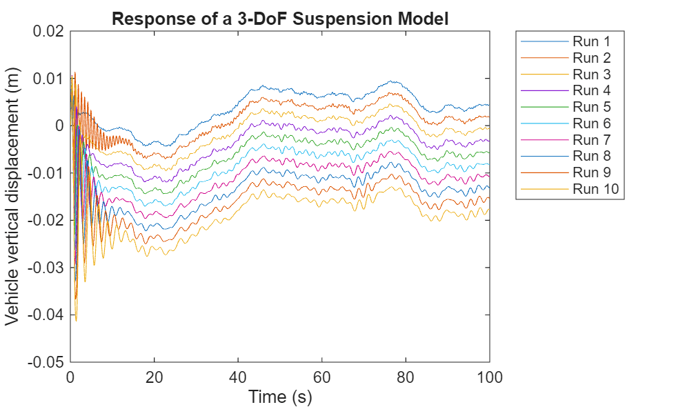
To see how varying the vehicle mass affects the vehicle dynamics, plot the vertical vehicle displacements.

1. Access the SimulationOutput object for each simulation. The SimulationOutput object contains a property for each type of logged data.

2. Access the logged signal data using dot notation. Within each SimulationOutput object, signal logging data and metadata are grouped in a Simulink.SimulationData.Dataset object with the default name of logsout.

3. Access the vertical_disp signal using getElement.

4. Access the timeseries object that contains the time and signal data for vertical_disp using the Values property of the vertical_disp signal.

5. Plot the results for each simulation.

legend_labels = cell(1,numSims);
for i = 1:numSims
    simout = out(i);
    ts = simout.logsout.getElement("vertical_disp").Values;
ts.plot;
    legend_labels{i} = "Run " + num2str(i);
    hold on
end
title("Response of a 3-DoF Suspension Model")
xlabel("Time (s)");
ylabel("Vehicle vertical displacement (m)");
legend(legend_labels,"Location","NorthEastOutside");

Close MATLAB Workers

Close the parallel pool.

delete(gcp("nocreate"));

Parallel pool using the 'Processes' profile is shutting down.