Algebraic Loop Concepts
An algebraic loop occurs when a signal loop in a model contains only blocks that have direct feedthrough. Direct feedthrough refers to blocks that use the input value for the current time step to calculate the output value for the current time step. A signal loop that contains only blocks with direct feedthrough creates a circular dependency of block output and input values in the same time step. The resulting equation is an algebraic equation that requires a solution at each time step and adds computational cost.
Some blocks always have direct feedthrough, while others have direct feedthrough only for certain block configurations. Examples of blocks with direct feedthrough include:
State-Space block with a nonzero D matrix
Transfer Fcn block with a numerator order that is the same as the denominator order
Zero-Pole block with the same number of zeros and poles
Blocks that do not have direct feedthrough maintain one or more state variables that store input values from prior time steps. Examples of blocks that do not have direct feedthrough include the Integrator block and the Unit Delay block.
Tip
To determine whether a block has direct feedthrough, refer to the Block Characteristics
table on the block reference page. To view the block characteristics for all blocks, use the
Block
Support Table block or the showblockdatatypetable function.
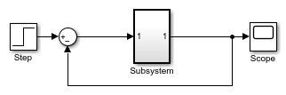
Consider a model that contains a Sum block that subtracts the block output value xa from the input value u.
The model implements this equation
xa = u – xa.
For this simple loop, the solution is xa = u/2.
Mathematical Interpretation
The software has several numerical solvers for simulating ordinary differential equations (ODEs). ODEs are systems of equations that you can write as
where x is the state vector and t is the independent time variable.
Some systems of equations include additional constraints that involve the independent variable and the state vector, but not the derivative of the state vector. Such systems are called differential algebraic equations (DAEs).
The term algebraic refers to equations that do not involve derivatives. You can express DAEs that arise in engineering in the semi-explicit form
where:
f and g can be vector functions.
The first equation is the differential equation.
The second equation is the algebraic equation.
The vector of differential variables is x.
The vector of algebraic variables is xa.
In a model, an algebraic loop represents an algebraic constraint. Models with algebraic loops define a system of differential algebraic equations. The software solves the algebraic loop numerically for xa at each step of a simulation that uses an ODE solver.
Consider this model that implements a simple system of DAEs. The inner loop represents an algebraic constraint, while the outer loop represents a differential equation.
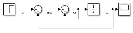
The model implements this system of DAEs.
x' = xa
0 = u - x - 2xa
For each step the ODE solver takes, the algebraic loop solver must solve the algebraic constraint for xa before calculating the derivative x'.
Physical Interpretation
Algebraic constraints:
Occur when modeling physical systems, often due to conservation laws, such as conservation of mass and energy
Occur when you choose a particular coordinate system for a model
Help impose design constraints on system responses in a dynamic system
Use Simscape™ to model systems that span mechanical, electrical, hydraulic, and other physical domains as physical networks. Simscape constructs the DAEs that characterize the behavior of a model. The software integrates these equations with the rest of the model and then solves the DAEs directly. Simulink® solves the variables for the components in the different physical domains simultaneously, avoiding problems with algebraic loops.
Artificial Algebraic Loops
An artificial algebraic loop occurs when an atomic subsystem or Model block causes Simulink to detect an algebraic loop, even though the contents of the subsystem do not contain a direct feedthrough from the input to the output. When you create an atomic subsystem, all Inport blocks are direct feedthrough, resulting in an algebraic loop.
Start with the included model, which represents a simple proportional control of the plant described by
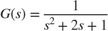
which can be rewritten in state-space form as
![$$ \dot{x} = \left[ \begin{array}{cc} -2 & -1 \\ 1 & 0 \end{array} \right] + \left( \begin{array}{c} 0\\1 \end{array} \right) $$](../../examples/simulink/win64/ArtifAlgLoopsExample_eq12603750421915334129.png)
![$$ y = \left[\begin{array}{cc}0&1\end{array}\right] $$](../../examples/simulink/win64/ArtifAlgLoopsExample_eq18346827941344727566.png)
The system has neither algebraic variables nor direct feedthrough and does not contain an algebraic loop.
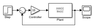
Modify the model as described in the following steps:
Enclose the Controller and Plant blocks in a subsystem.
In the subsystem dialog box, select Treat as atomic unit to make the subsystem atomic.
In the Diagnostics pane of the Model Configuration Parameters, set the Algebraic Loop parameter to
error.
When simulating this model, an algebraic loop occurs because the subsystem is direct feedthrough, even though the path within the atomic subsystem is not direct feedthrough. Simulation stops with an algebraic loop error.
How the Algebraic Loop Solver Works
When a model contains an algebraic loop, Simulink uses a nonlinear solver at each time step to solve the algebraic loop. The solver performs iterations to determine the solution to the algebraic constraint, if there is one. As a result, models with algebraic loops can run more slowly than models without algebraic loops.
Simulink uses a dogleg trust region algorithm to solve algebraic loops. The tolerance used
is smaller than the ODE solver Reltol and Abstol. This is
because Simulink uses the “explicit ODE method” to solve Index-1 differential algebraic equations
(DAEs).
For the algebraic loop solver to work,
There must be one block where the loop solver can break the loop and attempt to solve the loop.
The model should have real double signals.
The underlying algebraic constraint must be a smooth function
For example, suppose your model has a Sum block with two inputs—one additive, the other subtractive. If you feed the output of the Sum block to one of the inputs, you create an algebraic loop where all of the blocks include direct feedthrough.
The Sum block cannot compute the output without knowing the input. Simulink detects the algebraic loop, and the algebraic loop solver solves the loop using an iterative loop. In the Sum block example, the software computes the correct result this way:
| xa(t) = u(t) / 2. | (1) |
The algebraic loop solver uses a gradient-based search method, which requires continuous first derivatives of the algebraic constraint that correspond to the algebraic loop. As a result, if the algebraic loop contains discontinuities, the algebraic loop solver can fail.
For more information, see Solving Index-1 DAEs in MATLAB and Simulink 1
Trust-Region and Line-Search Algorithms in the Algebraic Loop Solver
The Simulink algebraic loop solver uses one of two algorithms to solve algebraic loops:
Trust-Region
Line-Search
By default, Simulink chooses the best algebraic loop solver and may switch between the two methods during simulation. To explicitly enable automatic algebraic loop solver selection for your model, at the MATLAB® command line, enter:
set_param(model_name, 'AlgebraicLoopSolver','Auto');
To switch to the trust-region algorithm, at the MATLAB command line, enter:
set_param(model_name, 'AlgebraicLoopSolver', 'TrustRegion');
If the algebraic loop solver cannot solve the algebraic loop with the trust-region algorithm, try simulating the model using the line-search algorithm.
To switch to the line-search algorithm, at the MATLAB command line, enter:
set_param(model_name, 'AlgebraicLoopSolver', 'LineSearch');
For more information, see:
Shampine and Reichelt’s nleqn.m code
The Fortran program HYBRD1 in the User Guide for MINPACK-1 2
Powell’s “A Fortran subroutine for solving systems in nonlinear equations,” in Numerical Methods for Nonlinear Algebraic Equations3
Trust-Region Methods for Nonlinear Minimization (Optimization Toolbox).
Line Search (Optimization Toolbox).
Limitations of the Algebraic Loop Solver
Algebraic loop solving is an iterative process. The Simulink algebraic loop solver is successful only if the algebraic loop converges to a definite answer. When the loop fails to converge, or converges too slowly, the simulation exits with an error.
The algebraic loop solver cannot solve algebraic loops that contain any of the following:
Blocks with discrete-valued outputs
Blocks with nondouble or complex outputs
Discontinuities
Stateflow® charts
These limitations also apply to artificial algebraic loops. For information about artificial algebraic loops, see Remove Algebraic Loops.
Implications of Algebraic Loops in a Model
If your model contains an algebraic loop:
You cannot generate code for the model.
The Simulink algebraic loop solver might not be able to solve the algebraic loop.
While Simulink is trying to solve the algebraic loop, the simulation can execute slowly.
For most models, the algebraic loop solver is computationally expensive for the first time step. Simulink solves subsequent time steps rapidly because a good starting point for xa is available from the previous time step.
See Also
Algebraic Constraint | Descriptor State-Space
Topics
1 Shampine, Lawrence F., M.W.Reichelt, and J.A.Kierzenka. ”Solving Index-1 DAEs in MATLAB and Simulink.”Siam Review.Vol.18,No.3,1999,pp.538–552.
2 More,J.J.,B.S.Garbow, and K.E.Hillstrom. User guide for MINPACK-1. Argonne, IL:Argonne National Laboratory,1980.
3 Rabinowitz, Philip, ed. Numerical Methods for Nonlinear Algebraic Equations, New York: Gordon and Breach Science Publishers, 1970.