linearize

Linear approximation of Simulink model or subsystem

Syntax

linsys = linearize(model,io)

linsys = linearize(model,io,op)

linsys = linearize(model,io,param)

linsys = linearize(model,io,blocksub)

linsys = linearize(model,io,options)

linsys = linearize(model,io,op,param,blocksub,options)

linsys = linearize(___,'StateOrder',stateorder)

[linsys,linop] = linearize(___)

[linsys,linop,info] = linearize(___)

Description

linsys = linearize(model,io) returns a linear approximation of the nonlinear Simulink^® model model at the model operating point using the analysis points specified in io. Using io, you can specify individual analysis points or you can specify a block or subsystem to linearize. If you omit io, then linearize uses the root-level inports and outports of the model as analysis points.

linsys = linearize(model,io,op) linearizes the model at operating point op.

linsys = linearize(model,io,param) linearizes the model using the parameter value variations specified in param. You can vary any model parameter with a value given by a variable in the model workspace, the MATLAB^® workspace, or a data dictionary.

linsys = linearize(model,io,blocksub) linearizes the model using the substitute block or subsystem linearizations specified in blocksub.

linsys = linearize(model,io,options) linearizes the model using additional linearization options.

linsys = linearize(model,io,op,param,blocksub,options) linearizes the model using any combination of op, param, blocksub, and options in any order.

linsys = linearize(___,'StateOrder',stateorder) specifies the order of the states in the linearized model for any of the previous syntaxes.

[linsys,linop] = linearize(___) returns the operating point at which the model was linearized. Use this syntax when linearizing at simulation snapshots or when varying parameters during linearization.

[linsys,linop,info] = linearize(___) returns additional linearization information. To select the linearization information to return in info, enable the corresponding option in options.

Examples

Linearize Model Using Specified I/O Set

Open the Simulink model.

mdl = 'watertank';
open_system(mdl)

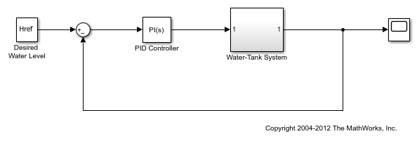
Specify a linearization input at the output of the PID Controller block, which is the input signal for the Water-Tank System block.

io(1) = linio('watertank/PID Controller',1,'input');

Specify a linearization output point at the output of the Water-Tank System block. Specifying the output point as open-loop removes the effects of the feedback signal on the linearization without changing the model operating point.

io(2) = linio('watertank/Water-Tank System',1,'openoutput');

Linearize the model using the specified I/O set.

linsys = linearize(mdl,io);

linsys is the linear approximation of the plant at the model operating point.

Linearize Model at Specified Operating Point

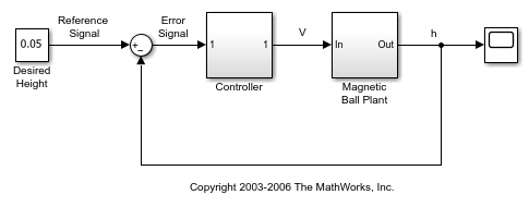
Open the Simulink model.

mdl = 'magball';
open_system(mdl)

Find a steady-state operating point at which the ball height is 0.05. Create a default operating point specification, and set the height state to a known value.

opspec = operspec(mdl);
opspec.States(5).Known = 1;
opspec.States(5).x = 0.05;

Trim the model to find the operating point.

options = findopOptions('DisplayReport','off');
op = findop(mdl,opspec,options);

Specify linearization input and output signals to compute the closed-loop transfer function.

io(1) = linio('magball/Desired Height',1,'input');
io(2) = linio('magball/Magnetic Ball Plant',1,'output');

Linearize the model at the specified operating point using the specified I/O set.

linsys = linearize(mdl,io,op);

Linearize Model at Simulation Snapshot Time

Open the Simulink model.

mdl = 'watertank';
open_system(mdl)

To compute the closed-loop transfer function, first specify the linearization input and output signals.

io(1) = linio('watertank/PID Controller',1,'input');
io(2) = linio('watertank/Water-Tank System',1,'output');

Simulate sys for 10 seconds and linearize the model.

linsys = linearize(mdl,io,10);

Batch Linearize Model for Parameter Variations

Open the Simulink model.

mdl = 'scdcascade';
open_system(mdl)

Specify parameter variations for the outer-loop controller gains, Kp1 and Ki1. Create parameter grids for each gain value.

Kp1_range = linspace(Kp1*0.8,Kp1*1.2,6);
Ki1_range = linspace(Ki1*0.8,Ki1*1.2,4);
[Kp1_grid,Ki1_grid] = ndgrid(Kp1_range,Ki1_range);

Create a parameter value structure with fields Name and Value.

params(1).Name = 'Kp1';
params(1).Value = Kp1_grid;
params(2).Name = 'Ki1';
params(2).Value = Ki1_grid;

params is a 6-by-4 parameter value grid, where each grid point corresponds to a unique combination of Kp1 and Ki1 values.

Define linearization input and output points for computing the closed-loop response of the system.

io(1) = linio('scdcascade/setpoint',1,'input');
io(2) = linio('scdcascade/Sum',1,'output');

Linearize the model at the model operating point using the specified parameter values.

linsys = linearize(mdl,io,params);

Specify Substitute Block Linearization and Linearize Model

Open the Simulink model.

mdl = 'scdpwm';
open_system(mdl)

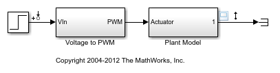
Extract linearization input and output from the model.

io = getlinio(mdl);

Linearize the model at the model operating point.

linsys = linearize(mdl,io)

linsys =
 
  D = 
                Step
   Plant Model     0
 
Static gain.

The discontinuities in the Voltage to PWM block cause the model to linearize to zero. To treat this block as a unit gain during linearization, specify a substitute linearization for this block.

blocksub.Name = 'scdpwm/Voltage to PWM';
blocksub.Value = 1;

Linearize the model using the specified block substitution.

linsys = linearize(mdl,blocksub,io)

linsys =
 
  A = 
                 State Space(  State Space(
   State Space(        0.9999       -0.0001
   State Space(        0.0001             1
 
  B = 
                   Step
   State Space(  0.0001
   State Space(   5e-09
 
  C = 
                State Space(  State Space(
   Plant Model             0             1
 
  D = 
                Step
   Plant Model     0
 
Sample time: 0.0001 seconds
Discrete-time state-space model.

Specify Sample Time of Linearized Model

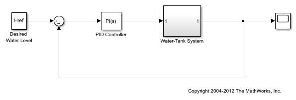
Open the Simulink model.

mdl = 'watertank';
open_system(mdl)

To linearize the Water-Tank System block, specify a linearization input and output.

io(1) = linio('watertank/PID Controller',1,'input');
io(2) = linio('watertank/Water-Tank System',1,'openoutput');

Create a linearization option set, and specify the sample time for the linearized model.

options = linearizeOptions('SampleTime',0.1);

Linearize the plant using the specified options.

linsys = linearize(mdl,io,options)

linsys =
 
  A = 
          H
   H  0.995
 
  B = 
      PID Controll
   H       0.02494
 
  C = 
                 H
   Water-Tank S  1
 
  D = 
                 PID Controll
   Water-Tank S             0
 
Sample time: 0.1 seconds
Discrete-time state-space model.

The linearized plant is a discrete-time state-space model with a sample time of 0.1.

Linearize Block or Subsystem at Model Operating Point

Open the Simulink model.

mdl = 'watertank';
open_system(mdl)

Specify the full block path for the block you want to linearize.

blockpath = 'watertank/Water-Tank System';

Linearize the specified block at the model operating point.

linsys = linearize(mdl,blockpath);

Linearize Block or Subsystem at Trimmed Operating Point

Open Simulink model.

mdl = 'magball';
open_system(mdl)

Find a steady-state operating point at which the ball height is 0.05. Create a default operating point specification, and set the height state to a known value.

opspec = operspec(mdl);
opspec.States(5).Known = 1;
opspec.States(5).x = 0.05;

options = findopOptions('DisplayReport','off');
op = findop(mdl,opspec,options);

Specify the block path for the block you want to linearize.

blockpath = 'magball/Magnetic Ball Plant';

Linearize the specified block at the specified operating point.

linsys = linearize(mdl,blockpath,op);

Specify State Order in Linearized Model

Open the Simulink model.

mdl = 'magball';
open_system(mdl)

Linearize the plant at the model operating point.

blockpath = 'magball/Magnetic Ball Plant';
linsys = linearize(mdl,blockpath);

View the default state order for the linearized plant.

linsys.StateName

ans =

  3×1 cell array

    {'height' }
    {'Current'}
    {'dhdt'   }

Linearize the plant and reorder the states in the linearized model. Set the rate of change of the height as the second state.

stateorder = {'magball/Magnetic Ball Plant/height';...
              'magball/Magnetic Ball Plant/dhdt';...
              'magball/Magnetic Ball Plant/Current'};
linsys = linearize(mdl,blockpath,'StateOrder',stateorder);

View the new state order.

linsys.StateName

ans =

  3×1 cell array

    {'height' }
    {'dhdt'   }
    {'Current'}

Linearize Model at Multiple Snapshot Times

Open the Simulink model.

mdl = 'watertank';
open_system(mdl)

To compute the closed-loop transfer function, first specify the linearization input and output signals.

io(1) = linio('watertank/PID Controller',1,'input');
io(2) = linio('watertank/Water-Tank System',1,'output');

Simulate sys and linearize the model at 0 and 10 seconds. Return the operating points that correspond to these snapshot times; that is, the operating points at which the model was linearized.

[linsys,linop] = linearize(mdl,io,[0,10]);

Batch Linearize Plant Model and Obtain Linearization Offsets

Open the Simulink model.

mdl = 'watertankNLModel';
open_system(mdl)

Specify the initial condition for water height.

h0 = 10;

Specify model linear analysis points.

io(1) = linio('watertankNLModel/Step',1,'input');
io(2) = linio('watertankNLModel/H',1,'output');

Simulate the model and extract operating points at time snapshots.

tlin = [0 30 40 50 60 70 80];
op = findop(mdl,tlin);

To store offsets during linearization, create a linearization option set and set StoreOffsets to "struct". Doing so returns the linearization offsets in the info output argument of linearize.

options = linearizeOptions(StoreOffsets="struct");

Batch linearize the plant at the trimmed operating points, using the specified I/O points and parameter variations.

[linsys,~,info] = linearize(mdl,io,op,options);
info.Offsets

ans=7×1 struct array with fields:
    dx
    x
    u
    y
    OutputName
    InputName
    StateName
    Ts

You can use the offsets in info.Offsets when configuring an LPV System block. This requires extracting offsets in the supported format using the using getOffsetsForLPV function. Additionally, when using the ssInterpolant function, you must explicitly specify info.Offsets as an additional input argument.

Alternatively, you can store offsets directly in the Offsets property of the linearized ss model. To do so, set StoreOffsets option to "system". (Since R2025a)

options.StoreOffsets = "system";
linsys2 = linearize(mdl,io,op,options);
linsys2.Offsets

ans=7×1 struct array with fields:
    dx
    x
    u
    y

Storing offsets directly with the system can simplify LPV modeling workflows and facilitate the comparison of the nonlinear and linearized responses of a Simulink® model. For an example on how you can use this system to build a linear parameter-varying model directly using ssInterpolant, see Create LPV Model from Batch Linearization Results.

Obtain Batch Linearization Results with Uniform State Consistency

Since R2025a

This example shows how to obtain an array of state-space models with uniform state consistency when using batch linearization. Building linear parameter-varying models (LPV) models from a state-space array obtained using batch linearization requires consistent and uniform state dimensions, delay modeling, and offset handling across the linearization grid.

For this example, consider a model of physical pendulum. The initial conditions for the pendulum angle is 45 degrees counterclockwise with zero applied torque. Additionally, the initial condition for the pendulum angular velocity is 0 deg/s. Specify the parameters and load the model.

tau0 = 0;
mgl = 1;
inv_inert = 1;
c = 0.1;
theta0 = pi/4;
dtheta0 = 0;
mdl = "scdPendulumNoWrap";
load_system(mdl);

In this example, set the linearization to not treat the Saturation block as gain. The Saturation block in this model limits the total torque input between the values -1 and 1. Therefore, linearization will analytically linearize this block to zero if the signal input value lies outside this range.

set_param(mdl+"/clip","LinearizeAsGain","off");

Specify the input to the Saturation block as linearization input and theta as output.

io(1) = linio(mdl+"/tau0",1,"input");
io(2) = linio(mdl+"/pendulum",1,"output");

Create two operating points for linearization. For the second operating point, specify an input level that lies outside the saturation range.

op1 = operpoint(mdl);
op2 = copy(op1);
op2.Inputs(1).u = 2;
op = [op1,op2];

First, linearize the system with the BatchConsistency option set to false.

lin_opt = linearizeOptions(StoreOffsets="system",BlockReduction="on",BatchConsistency=false);
sys = linearize(mdl,io,op,lin_opt);
sys

sys(:,:,1,1) =
 
  A = 
                  theta  theta_dot
   theta              0          1
   theta_dot    -0.7071       -0.1
 
  B = 
              tau0
   theta         0
   theta_dot     1
 
  C = 
                     theta  theta_dot
   pendulum/the          1          0
 
  D = 
                 tau0
   pendulum/the     0
 

sys(:,:,2,1) =
 
  D = 
                 tau0
   pendulum/the     0
 
2x1 array of continuous-time state-space models.
Model Properties

The batch linearization result returns a 2-by-1 array of state-space models corresponding to the defined operating points. The first model in the array has two states but the second model linearizes to zero because the input level lies outside the saturation range. When BatchConsistency is disabled, linearization reduces each model in the array to the maximum extent.

Now, enable the BatchConsistency option and linearize the model again at the same operating conditions.

lin_optc = linearizeOptions(StoreOffsets="system",BlockReduction="on",BatchConsistency=true);
sysc = linearize(mdl,io,op,lin_optc);
sysc

sysc(:,:,1,1) =
 
  A = 
                  theta  theta_dot
   theta              0          1
   theta_dot    -0.7071       -0.1
 
  B = 
              tau0
   theta         0
   theta_dot     1
 
  C = 
                     theta  theta_dot
   pendulum/the          1          0
 
  D = 
                 tau0
   pendulum/the     0
 

sysc(:,:,2,1) =
 
  A = 
                  theta  theta_dot
   theta              0          1
   theta_dot    -0.7071       -0.1
 
  B = 
              tau0
   theta         0
   theta_dot     0
 
  C = 
                     theta  theta_dot
   pendulum/the          1          0
 
  D = 
                 tau0
   pendulum/the     0
 
2x1 array of continuous-time state-space models.
Model Properties

The batch linearization now produces an array where both models have two states. When you enable BatchConsistency, linearization removes only the states and delays that do not contribute to the input-output map for all models in the batch linearization array, and hence preserves consistency across all models. This is particularly helpful when building gridded LPV models.

For an example that show how to build an LPV model for this pendulum, see Create LPV Pendulum Model Using Batch Linearization.

Model Fractional Delays During Discretization

Since R2025a

This example shows how to model extra delays that arise during discretization. Typically, discretizing models with input or output delays that are not integer multiples of the model sample time can give rise to additional delays besides the discrete input and output delays. linearize allows you to specify whether you want to model these delays as internal delays or additional states.

Consider a simple Simulink® model, containing an LTI system with two states and an input delay of 2.7 seconds.

sys = tf([1,2],[1,4,2],InputDelay=2.7);
mdl = "linDelayModeling";
load_system(mdl)

Linearize the model with a sample time of 1 second. Additionally, set the discretization method to Tustin and specify a third Thiran filter to model the fractional delay.

opt = linearizeOptions(...
    SampleTime=1,...
    UseExactDelayModel=true);
opt.RateConversionOptions.Method = "tustin";
opt.RateConversionOptions.ThiranOrder = 3;
linsys = linearize(mdl,opt)

linsys =
 
  A = 
              ?          ?          ?          ?          ?
   ?    -0.4286    -0.5714   -0.00265    0.06954      2.286
   ?     0.2857     0.7143  -0.001325    0.03477      1.143
   ?          0          0    -0.2432     0.1449    -0.1153
   ?          0          0       0.25          0          0
   ?          0          0          0      0.125          0
 
  B = 
            in
   ?  0.002058
   ?  0.001029
   ?         8
   ?         0
   ?         0
 
  C = 
                ?          ?          ?          ?          ?
   out     0.2857     0.7143  -0.001325    0.03477      1.143
 
  D = 
              in
   out  0.001029
 
Sample time: 1 seconds
Discrete-time state-space model.
Model Properties

Linearization returns the discretized model containing three additional states corresponding to a third-order Thiran filter. Since the time delay divided by the sample time is 2.7, the third-order Thiran filter can approximate the entire time delay. In the linearization options opt, the opt.RateConversionOptions.DelayModeling property determines how to model extra delays. By default, it is set to "state" and models extra delays as extra states. To model extra delays as internal model delays instead, you can set DelayModeling to "delay".

opt.RateConversionOptions.DelayModeling = "delay";

Linearize the model again.

linsys2 = linearize(mdl,opt)

linsys2 =
 
  A = 
            ?        ?
   ?  -0.4286  -0.5714
   ?   0.2857   0.7143
 
  B = 
          in
   ?  0.5714
   ?  0.2857
 
  C = 
             ?       ?
   out  0.2857  0.7143
 
  D = 
            in
   out  0.2857
 
  (values computed with all internal delays set to zero)

  Internal delays (sampling periods): 1  1  1 
 
Sample time: 1 seconds
Discrete-time state-space model.
Model Properties

The linearization now models extra delays as internal delays in the discretized model.

Input Arguments

model — Simulink model name

character vector | string

Simulink model name, specified as a character vector or string. The model must be in the current working folder or on the MATLAB path.

io — Analysis points

linearization I/O object | vector of linearization I/O objects | string | character vector

Analysis points for linearizing model, specified as one of the following:

• Linearization I/O object or a vector of linearization I/O objects — Specify a list of one or more inputs, outputs, and loop openings. To create the list of analysis points:

  • Define the inputs, outputs, and openings using the linio function.

  • If the inputs, outputs, and openings are specified in the Simulink model, extract these points from the model using the getlinio function.

• String or character vector — Specify the full path of a block or subsystem to linearize. The software treats the inports and outports of the specified block as open-loop inputs and outputs, which isolates the block from the rest of the model before linearization.

The analysis points defined in io must correspond to the Simulink model model or some normal-mode model reference in the model hierarchy.

If you omit io, then linearize uses the root-level inports and outports of the model as analysis points.

For more information on specifying linearization inputs, outputs, and openings, see Specify Portion of Model to Linearize.

op — Operating point

OperatingPoint object | array of OperatingPoint objects | vector of positive scalars

Operating point for linearization, specified as one of the following:

• OperatingPoint object, created using:

  • operpoint

  • findop with either a single operating point specification, or a single snapshot time.

• Array of OperatingPoint objects, specifying multiple operating points. To create an array of OperatingPoint objects, you can:

  • Extract operating points at multiple snapshot times using findop.

  • Batch trim your model using multiple operating point specifications. For more information, see Batch Compute Steady-State Operating Points for Multiple Specifications.

  • Batch trim your model using parameter variations. For more information, see Batch Compute Steady-State Operating Points for Parameter Variation.

• Vector of positive scalars representing one or more simulation snapshot times. The software simulates sys and linearizes the model at the specified snapshot times.

  If you also specify parameter variations using param, the software simulates the model for each snapshot time and parameter grid point combination. This operation can be computationally expensive.

If you specify parameter variations using param, and the parameters:

• Affect the model operating point, then specify op as an array of operating points with the same dimensions as the parameter value grid. To obtain the operating points that correspond to the parameter value combinations, batch trim your model using param before linearization. For more information, see Batch Linearize Model at Multiple Operating Points Derived from Parameter Variations.

• Do not affect the model operating point, then specify op as a single operating point.

blocksub — Substitute linearizations for blocks and subsystems

structure | structure array

Substitute linearizations for blocks and subsystems, specified as a structure or an n-by-1 structure array, where n is the number of blocks for which you want to specify a linearization. Use blocksub to specify a custom linearization for a block or subsystem. For example, you can specify linearizations for blocks that do not have analytic linearizations, such as blocks with discontinuities or triggered subsystems.

To study the effects of varying the linearization of a block on the model dynamics, you can batch linearize your model by specifying multiple substitute linearizations for a block.

If you substitute a linearization with a sample time that differs from that of the original block or subsystem, it is best practice to set the overall linearization sample time (options.SampleTime) to a nondefault value.

Each substitute linearization structure has the following fields.

Name — Block path

character vector | string

Block path of the block for which you want to specify the linearization, specified as a character vector or string.

Value — Substitute linearization

double | double array | LTI model | model array | structure

Substitute linearization for the block, specified as one of the following:

• Double — Specify the linearization of a SISO block as a gain.

• Array of doubles — Specify the linearization of a MIMO block as an n_u-by-n_y array of gain values, where n_u is the number of inputs and n_y is the number of outputs.

• LTI model, uncertain state-space model, or uncertain real object — The I/O configuration of the specified model must match the configuration of the block specified by Name. Using an uncertain model requires Robust Control Toolbox™ software.

• Array of LTI models, uncertain state-space models, or uncertain real objects — Batch linearize the model using multiple block substitutions. The I/O configuration of each model in the array must match the configuration of the block for which you are specifying a custom linearization. If you:

  • Vary model parameters using param and specify Value as a model array, the dimensions of Value must match the parameter grid size.

  • Specify op as an array of operating points and Value as a model array, the dimensions of Value must match the size of op.

  • Define block substitutions for multiple blocks, and specify Value as an array of LTI models for one or more of these blocks, the dimensions of the arrays must match.

• Structure with the following fields.

  Field	Description
  Specification	Block linearization, specified as a character vector that contains one of the following: MATLAB expression Name of a Custom Linearization Function in your current working folder or on the MATLAB path The specified expression or function must return one of the following: Linear model in the form of a D-matrix Control System Toolbox™ LTI model object Uncertain state-space model or uncertain real object (requires Robust Control Toolbox software) The I/O configuration of the returned model must match the configuration of the block specified by Name.
  Type	Specification type, specified as one of the following: 'Expression' 'Function'
  ParameterNames	Linearization function parameter names, specified as a cell array of character vectors. Specify ParameterNames only when Type = 'Function' and your block linearization function requires input parameters. These parameters only impact the linearization of the specified block. You must also specify the corresponding blocksub.Value.ParameterValues field.
  ParameterValues	Linearization function parameter values, specified as a vector of doubles. The order of parameter values must correspond to the order of parameter names in blocksub.Value.ParameterNames. Specify ParameterValues only when Type = 'Function' and your block linearization function requires input parameters.

param — Parameter samples

structure | structure array

Parameter samples for linearization, specified as one of the following:

• Structure — Vary the value of a single parameter by specifying parameters as a structure with the following fields.

  • Name — Parameter name, specified as a character vector or string. You can specify any model parameter that is a variable in the model workspace, the MATLAB workspace, or a data dictionary. If the variable used by the model is not a scalar variable, specify the parameter name as an expression that resolves to a numeric scalar value. For example, use the first element of vector V as a parameter.

    parameters.Name = 'V(1)';

  • Value — Parameter sample values, specified as a double array.

  For example, vary the value of parameter A in the 10% range.

  parameters.Name = 'A';
  parameters.Value = linspace(0.9*A,1.1*A,3);

• Structure array — Vary the value of multiple parameters. For example, vary the values of parameters A and b in the 10% range.

  [A_grid,b_grid] = ndgrid(linspace(0.9*A,1.1*A,3),...
                           linspace(0.9*b,1.1*b,3));
  parameters(1).Name = 'A';
  parameters(1).Value = A_grid;
  parameters(2).Name = 'b';
  parameters(2).Value = b_grid;

For more information, see Specify Parameter Samples for Batch Linearization.

If param specifies tunable parameters only, the software batch linearizes the model using a single model compilation.

To compute the offsets required by the LPV System block, specify param, and set options.StoreOffsets to true. You can then return additional linearization information in info, and extract the offsets using getOffsetsForLPV.

stateorder — State order in linearization results

cell array of character vectors

State order in linearization results, specified as a cell array of block paths or state names. The order of the block paths and states in stateorder indicates the order of the states in linsys.

You can specify block paths for any blocks in model that have states, or any named states in model.

You do not have to specify every block and state from model in stateorder. The states you specify appear first in linsys, followed by the remaining states in their default order.

options — Linearization algorithm options

linearizeOptions option set

Linearization algorithm options, specified as a linearizeOptions option set.

Output Arguments

linsys — Linearization result

state-space model | array of state-space models

Linearization result, returned as a state-space model or an array of state-space models.

For most models, linsys is returned as an ss object or an array of ss objects. However, if model contains one of the following blocks in the linearization path defined by io, then linsys returns the specified type of state-space model.

Block	linsys Type
Block with a substitution specified as a genss object or tunable model object	genss
Block with a substitution specified as an uncertain model, such as uss	uss (Robust Control Toolbox)
Sparse Second Order block	mechss
Descriptor State-Space block configured to linearize to a sparse model	sparss

The dimensions of linsys depend on the specified parameter variations and block substitutions, and the operating points at which you linearize the model.

Note

If you specify more than one of op, param, or blocksub.Value as an array, then their dimensions must match.

Parameter Variation	Block Substitution	Linearize At...	Resulting linsys Dimensions
No parameter variation	No block substitution	Model operating point	Single state-space model
		Single operating point, specified as an OperatingPoint object or snapshot time using op
		N1-by-...-by-Nm array of OperatingPoint objects, specified by op	N1-by-...-by-Nm
		Ns snapshots, specified as a vector of snapshot times using op	Column vector of length Ns
	N1-by-...-by-Nm model array for at least one block, specified by blocksub.Value	Model operating point	N1-by-...-by-Nm
		Single operating point, specified as an OperatingPoint object or snapshot time using op
		N1-by-...-by-Nm array of operating points, specified as an array of OperatingPoint objects using op
		Ns snapshots, specified as a vector of snapshot times using op	Ns-by-N1-by-...-by-Nm
N1-by-...-by-Nm parameter grid, specified by param	Either no block substitution or an N1-by-...-by-Nm model array for at least one block, specified by blocksub.Value	Model operating point	N1-by-...-by-Nm
		Single operating point, specified as an OperatingPoint object or snapshot time using op
		N1-by-...-by-Nm array of OperatingPoint objects, specified by op
		Ns snapshots, specified as a vector of snapshot times using op	Ns-by-N1-by-...-by-Nm

For example, suppose:

• op is a 4-by-3 array of OperatingPoint objects and you do not specify parameter variations or block substitutions. In this case, linsys is a 4-by-3 model array.

• op is a single OperatingPoint object and param specifies a 3-by-4-by-2 parameter grid. In this case, linsys is a 3-by-4-by-2 model array.

• op is a row vector of positive scalars with two elements and you do not specify param. In this case, linsys is a column vector with two elements.

• op is a column vector of positive scalars with three elements and param specifies a 5-by-6 parameter grid. In this case, linsys is a 3-by-5-by-6 model array.

• op is a single operating point object, you do not specify parameter variations, and blocksub.Value is a 2-by-3 model array for one block in the model. In this case, linsys is a 2-by-3 model array.

• op is a column vector of positive scalars with four elements, you do not specify parameter variations, and blocksub.Value is a 1-by-2 model array for one block in the model. In this case, linsys is a 4-by-1-by-2 model array.

For more information on model arrays, see Model Arrays.

linop — Operating point

OperatingPoint object | array of OperatingPoint objects

Operating point at which the model was linearized, returned as an OperatingPoint object or an array of OperatingPoint objects with the same dimensions as linsys. Each element of linop is the operating point at which the corresponding linsys model was obtained.

If you specify op as a single OperatingPoint object or an array of OperatingPoint objects, then linop is a copy of op. If you specify op as a single operating point object and also specify parameter variations using param, then linop is an array with the same dimensions as the parameter grid. In this case, the elements of linop are scalar expanded copies of op.

To determine whether the model was linearized at a reasonable operating point, view the states and inputs in linop.

info — Linearization information

structure

Linearization information, returned as a structure with the following fields:

Offsets — Linearization offsets

[] (default) | structure | structure array

Linearization offsets that correspond to the operating point at which the model was linearized, returned as [] if options.StoreOffsets is "none". If options.StoreOffsets is "struct", Offsets is returned as one of the following:

• If linsys is a single state-space model, then Offsets is a structure.

• If linsys is an array of state-space models, then Offsets is a structure array with the same dimensions as linsys.

Each offset structure has the following fields:

Field	Description
x	State offsets used for linearization, returned as a column vector of length nx, where nx is the number of states in linsys.
y	Output offsets used for linearization, returned as a column vector of length ny, where ny is the number of outputs in linsys.
u	Input offsets used for linearization, returned as a column vector of length nu, where nu is the number of inputs in linsys.
dx	Derivative offsets for continuous time systems or updated state values for discrete-time systems, returned as a column vector of length nx.
StateName	State names, returned as a cell array that contains nx elements that match the names in linsys.StateName.
InputName	Input names, returned as a cell array that contains nu elements that match the names in linsys.InputName.
OutputName	Output names, returned as a cell array that contains ny elements that match the names in linsys.OutputName.
Ts	Sample time of the linearized system, returned as a scalar that matches the sample time in linsys.Ts. For continuous-time systems, Ts is 0.

If Offsets is a structure array, you can configure an LPV System block using the offsets. To do so, first convert them to the required format using getOffsetsForLPV. For an example, see Approximate Nonlinear Behavior Using Array of LTI Systems.

Additionally, if you want to return offsets directly in the Offsets property of the ss and sparss models, set options.StoreOffsets to "system". (since R2025a)

Advisor — Linearization diagnostic information

[] (default) | LinearizationAdvisor object | array of LinearizationAdvisor objects

Linearization diagnostic information, returned as [] if options.StoreAdvisor is false. Otherwise, Advisor is returned as one of the following:

• If linsys is a single state-space model, Advisor is a LinearizationAdvisor object.

• If linsys is an array of state-space models, Advisor is an array of LinearizationAdvisor objects with the same dimensions as linsys.

LinearizationAdvisor objects store linearization diagnostic information for individual linearized blocks. For an example of troubleshooting linearization results using a LinearizationAdvisor object, see Troubleshoot Linearization Results at Command Line.

Limitations

• Linearization is not supported for model hierarchies that contain referenced models configured to use a local solver.

• Linearization is not supported for Simscape™ networks configured to use a local solver.

More About

Custom Linearization Function

You can specify a substitute linearization for a block or subsystem in your Simulink model using a custom function on the MATLAB path.

Your custom linearization function must have one BlockData input argument, which is a structure that the software creates and passes to the function. BlockData has the following fields:

Field	Description
BlockName	Name of the block for which you are specifying a custom linearization.
Parameters	Block parameter values, specified as a structure array with Name and Value fields. Parameters contains the names and values of the parameters you specify in the blocksub.Value.ParameterNames and blocksub.Value.ParameterValues fields.
Inputs	Input signals to the block for which you are defining a linearization, specified as a structure array with one structure for each block input. Each structure in Inputs has the following fields: Field Description BlockName Full block path of the block whose output connects to the corresponding block input. PortIndex Output port of the block specified by BlockName that connects to the corresponding block input. Values Value of the signal specified by BlockName and PortIndex. If this signal is a vector signal, then Values is a vector with the same dimension.
ny	Number of output channels of the block linearization.
nu	Number of input channels of the block linearization.
BlockLinearization	Current default linearization of the block, specified as a state-space model. You can specify a block linearization that depends on the default linearization using BlockLinearization.

Your custom function must return a model with nu inputs and ny outputs. This model must be one of the following:

• Linear model in the form of a D-matrix

• Control System Toolbox LTI model object

• Uncertain state-space model or uncertain real object (requires Robust Control Toolbox software)

For example, the following function multiplies the current default block linearization, by a delay of Td = 0.5 seconds. The delay is represented by a Thiran filter with sample time Ts = 0.1. The delay and sample time are parameters stored in BlockData.

function sys = myCustomFunction(BlockData)
    Td = BlockData.Parameters(1).Value;
    Ts = BlockData.Parameters(2).Value;
    sys = BlockData.BlockLinearization*Thiran(Td,Ts);
end 

Save this function to a location on the MATLAB path.

To use this function as a custom linearization for a block or subsystem, specify the blocksub.Value.Specification and blocksub.Value.Type fields.

blocksub.Value.Specification = 'myCustomFunction';
blocksub.Value.Type = 'Function';

To set the delay and sample time parameter values, specify the blocksub.Value.ParameterNames and blocksub.Value.ParameterValues fields.

blocksub.Value.ParameterNames = {'Td','Ts'};
blocksub.Value.ParameterValues = [0.5 0.1];

Algorithms

Model Properties for Linearization

By default, linearize automatically sets the following Simulink model properties.

• BufferReuse = 'off'

• BlockReductionOpt = 'off'

• SaveFormat = 'StructureWithTime'

After linearization, Simulink restores the original model properties.

Block-by-Block Linearization

Simulink Control Design™ software linearizes models using a block-by-block approach. The software individually linearizes each block in your Simulink model and produces the linearization of the overall system by combining the individual block linearizations.

The software determines the input and state levels for each block from the operating point, and obtains the Jacobian for each block at these levels.

For some blocks, the software cannot compute an analytical linearization in this manner. For example:

• Some nonlinearities do not have a defined Jacobian.

• Some discrete blocks, such as state charts and triggered subsystems, tend to linearize to zero.

• Some blocks do not implement a Jacobian.

• Custom blocks, such as S-Function blocks and MATLAB Function blocks, do not have analytical Jacobians.

You can specify a custom linearization for any such blocks for which you know the expected linearization. If you do not specify a custom linearization, the software linearizes the model by perturbing the block inputs and states and measuring the response to these perturbations. For each input and state, the default perturbation level is:

• $${10}^{-5}\left(1+\left|x\right|\right)$$ for double-precision values.

• $$0.005\left(1+\left|x\right|\right)$$ for single-precision values.

Here, x is the value of the corresponding input or state at the operating point. For information on how to change perturbation levels for individual blocks, see Change Perturbation Level of Blocks Perturbed During Linearization.

For more information, see Linearize Nonlinear Models and Exact Linearization Algorithm.

Full-Model Numerical Perturbation

You can linearize your system using full-model numerical perturbation, where the software computes the linearization of the full model by perturbing the values of root-level inputs and states. To do so, create a linearizeOptions object and set the LinearizationAlgorithm property to one of the following:

• 'numericalpert' — Perturb the inputs and states using forward differences; that is, by adding perturbations to the input and state values. This perturbation method is typically faster than the 'numericalpert2' method.

• 'numericalpert2' — Perturb the inputs and states using central differences; that is, by perturbing the input and state values in both positive and negative directions. This perturbation method is typically more accurate than the 'numericalpert' method.

For each input and state, the software perturbs the model and computes a linear model based on the model response to these perturbations. You can configure the state and input perturbation levels using the NumericalPertRel linearization options.

Block-by-block linearization has several advantages over full-model numerical perturbation:

• Most Simulink blocks have a preprogrammed linearization that provides an exact linearization of the block.

• You can use linear analysis points to specify a portion of the model to linearize.

• You can configure blocks to use custom linearizations without affecting your model simulation.

• Structurally nonminimal states are automatically removed.

• You can specify linearizations that include uncertainty (requires Robust Control Toolbox software).

• You can obtain detailed diagnostic information.

• When linearizing multirate models, you can use different rate conversion methods. Full-model numerical perturbation can only use zero-order-hold rate conversion.

For more information, see Linearize Nonlinear Models and Exact Linearization Algorithm.

Alternatives

As an alternative to the linearize function, you can linearize models using one of the following methods.

• To interactively linearize models, use the Model Linearizer app. For an example, see Linearize Simulink Model at Model Operating Point.

• To obtain multiple transfer functions without modifying the model or creating an analysis point set for each transfer function, use an slLinearizer interface. For an example, see Vary Parameter Values and Obtain Multiple Transfer Functions.

Although both Simulink Control Design software and the Simulink linmod function perform block-by-block linearization, Simulink Control Design linearization functionality has a more flexible user interface and uses Control System Toolbox numerical algorithms. For more information, see Linearization Using Simulink Control Design Versus Simulink.

Version History

Introduced in R2006a

R2025a: Improvements to sparse and descriptor state-space linearization, discrete rate conversion, offset handling, and state consistency

The linearization tools available in Simulink Control Design software now provide the following enhancements for linearization:

• Sparse linearization — The software can now return a first-order sparse (sparss) model without relying on block substitution for sparse-capable blocks. Previously, you could only perform sparse linearization when BlockReduction option of linearizeOptions and slTunerOptions was set to "on".

• Enhanced rate conversion options — The linearizeOptions and slTunerOptions objects now store the rate conversion related options under the new RateConversionOptions property. Additionally, rate conversion options now include DelayModeling and ThiranOrder. The DelayModeling option allows you to specify whether to model extra delays from discretization as internal delays or additional states. The ThiranOrder option specifies the order of the Thiran filter used to approximate fractional delays in the Tustin discretization. To set these properties, use dot notation:

  opt = linearizeOptions;
  opt.RateConversionOptions.Method = "tustin";
  opt.RateConversionOptions.DelayModeling = "delay";
  opt.RateConversionOptions.ThiranOrder = 3;

• Offset computation and storage — The software now allows you to directly store offsets in the Offsets property of the linearized ss and sparss models using the new value "system" for the option.

  opt = linearizeOptions(StoreOffsets="system")

  Additionally, you can now compute offsets during snapshot linearization. Calculation of offsets during simulation are limited to continuous time blocks and linear discrete time blocks. For example:

  tsnap = 7.5;
  sys = linearize(mdl,io,tsnap,opt);

• Consistent block reduction — When performing batch linearization, you can now use the new BatchConsistency option of linearizeOptions and slTunerOptions to only reduce the states that are reducible for all models in the grid of operating points. In addition, the software maintains this consistency during any rate conversion or delay modeling.

These changes also simplify LPV modeling workflows. Building LPV models in MATLAB and Simulink require consistent and uniform state dimensions, delay modeling, and offset handling across the linearization grid. For more information about building LPV models from batch linearization results, see ssInterpolant.

R2025a: linearizeOptions: Offset and rate conversion options changed

As a result of improvements to linearization workflows, how you specify options related to offsets and rate conversion in linearizeOptions has changed. This table describes the change in the workflow.

Before R2025a	R2025a
Offsets Do not compute linearization offsets. opt.StoreOffsets = "off"; Compute linearization offsets and return as an output argument of linearize. opt.StoreOffsets = "on"; [sys,~,info] = linearize(__,opt); offsets = info.Offsets;	Offsets Do not compute linearization offsets. opt.StoreOffsets = "none"; Compute linearization offsets and return as an output argument of linearize. opt.StoreOffsets = "struct"; [sys,~,info] = linearize(__,opt); offsets = info.Offsets;
Rate conversion Rate conversion method opt.RateConversionMethod = "tustin"; Prewarp frequency opt.PreWarpFreq = 10;	Rate conversion Rate conversion method opt.RateConversionOptions.Method = "tustin"; Prewarp frequency opt.RateConversionOptions.PreWarpFreq = 10;

R2020b: Linearize Simulink model to a sparse state-space model

You can linearize and obtain a sparse model from a Simulink model that contains a Sparse Second Order or Descriptor State-Space block.

• mechss model when you use a Sparse Second Order in your Simulink model.

• sparss model when you use a Descriptor State-Space block and select the Linearize to sparse model block parameter.

For more information, see Sparse Model Basics. For an example, see Linearize Simulink Model to a Sparse Second-Order Model Object.

R2016b: Compute operating point offsets for model inputs, outputs, states, and state derivatives during linearization

You can compute operating point offsets for model inputs, outputs, states, and state derivatives when linearizing Simulink models. Thee offsets streamline the creation of linear parameter-varying (LPV) systems.

To obtain operating point offsets, first create a linearizeOptions object and set the StoreOffsets option to true. Then, linearize the model.

You can extract the offsets from the info output argument and convert them into the required format for the LPV System block using the getOffsetsForLPV function.

R2014a: Block substitution input argument

You can specify a substitute linearization for a Simulink block or subsystem using the blocksub input argument of the linearize function.