Main Content

ClassificationNeuralNetwork

Neural network model for classification

Since R2021a

    Description

    A ClassificationNeuralNetwork object is a trained, feedforward, and fully connected neural network for classification. The first fully connected layer of the neural network has a connection from the network input (predictor data X), and each subsequent layer has a connection from the previous layer. Each fully connected layer multiplies the input by a weight matrix (LayerWeights) and then adds a bias vector (LayerBiases). An activation function follows each fully connected layer (Activations and OutputLayerActivation). The final fully connected layer and the subsequent softmax activation function produce the network's output, namely classification scores (posterior probabilities) and predicted labels. For more information, see Neural Network Structure.

    Creation

    Create a ClassificationNeuralNetwork object by using fitcnet.

    Properties

    expand all

    Neural Network Properties

    This property is read-only.

    Sizes of the fully connected layers in the neural network model, returned as a positive integer vector. The ith element of LayerSizes is the number of outputs in the ith fully connected layer of the neural network model.

    LayerSizes does not include the size of the final fully connected layer. This layer always has K outputs, where K is the number of classes in Y.

    Data Types: single | double

    This property is read-only.

    Learned layer weights for the fully connected layers, returned as a cell array. The ith entry in the cell array corresponds to the layer weights for the ith fully connected layer. For example, Mdl.LayerWeights{1} returns the weights for the first fully connected layer of the model Mdl.

    LayerWeights includes the weights for the final fully connected layer.

    Data Types: cell

    This property is read-only.

    Learned layer biases for the fully connected layers, returned as a cell array. The ith entry in the cell array corresponds to the layer biases for the ith fully connected layer. For example, Mdl.LayerBiases{1} returns the biases for the first fully connected layer of the model Mdl.

    LayerBiases includes the biases for the final fully connected layer.

    Data Types: cell

    This property is read-only.

    Activation functions for the fully connected layers of the neural network model, returned as a character vector or cell array of character vectors with values from this table.

    ValueDescription
    'relu'

    Rectified linear unit (ReLU) function — Performs a threshold operation on each element of the input, where any value less than zero is set to zero, that is,

    f(x)={x,x00,x<0

    'tanh'

    Hyperbolic tangent (tanh) function — Applies the tanh function to each input element

    'sigmoid'

    Sigmoid function — Performs the following operation on each input element:

    f(x)=11+ex

    'none'

    Identity function — Returns each input element without performing any transformation, that is, f(x) = x

    • If Activations contains only one activation function, then it is the activation function for every fully connected layer of the neural network model, excluding the final fully connected layer. The activation function for the final fully connected layer is always softmax (OutputLayerActivation).

    • If Activations is an array of activation functions, then the ith element is the activation function for the ith layer of the neural network model.

    Data Types: char | cell

    This property is read-only.

    Activation function for the final fully connected layer, returned as 'softmax'. The function takes each input xi and returns the following, where K is the number of classes in the response variable:

    f(xi)=exp(xi)j=1Kexp(xj).

    The results correspond to the predicted classification scores (or posterior probabilities).

    This property is read-only.

    Parameter values used to train the ClassificationNeuralNetwork model, returned as a NeuralNetworkParams object. ModelParameters contains parameter values such as the name-value arguments used to train the neural network classifier.

    Access the properties of ModelParameters by using dot notation. For example, access the function used to initialize the fully connected layer weights of a model Mdl by using Mdl.ModelParameters.LayerWeightsInitializer.

    Convergence Control Properties

    This property is read-only.

    Convergence information, returned as a structure array.

    FieldDescription
    IterationsNumber of training iterations used to train the neural network model
    TrainingLossTraining cross-entropy loss for the returned model, or resubLoss(Mdl,'LossFun','crossentropy') for model Mdl
    GradientGradient of the loss function with respect to the weights and biases at the iteration corresponding to the returned model
    StepStep size at the iteration corresponding to the returned model
    TimeTotal time spent across all iterations (in seconds)
    ValidationLossValidation cross-entropy loss for the returned model
    ValidationChecksMaximum number of times in a row that the validation loss was greater than or equal to the minimum validation loss
    ConvergenceCriterionCriterion for convergence
    HistorySee TrainingHistory

    Data Types: struct

    This property is read-only.

    Training history, returned as a table.

    ColumnDescription
    IterationTraining iteration
    TrainingLossTraining cross-entropy loss for the model at this iteration
    GradientGradient of the loss function with respect to the weights and biases at this iteration
    StepStep size at this iteration
    TimeTime spent during this iteration (in seconds)
    ValidationLossValidation cross-entropy loss for the model at this iteration
    ValidationChecksRunning total of times that the validation loss is greater than or equal to the minimum validation loss

    Data Types: table

    This property is read-only.

    Solver used to train the neural network model, returned as 'LBFGS'. To create a ClassificationNeuralNetwork model, fitcnet uses a limited-memory Broyden-Fletcher-Goldfarb-Shanno quasi-Newton algorithm (LBFGS) as its loss function minimization technique, where the software minimizes the cross-entropy loss.

    Predictor Properties

    This property is read-only.

    Predictor variable names, returned as a cell array of character vectors. The order of the elements of PredictorNames corresponds to the order in which the predictor names appear in the training data.

    Data Types: cell

    This property is read-only.

    Categorical predictor indices, returned as a vector of positive integers. Assuming that the predictor data contains observations in rows, CategoricalPredictors contains index values corresponding to the columns of the predictor data that contain categorical predictors. If none of the predictors are categorical, then this property is empty ([]).

    Data Types: double

    This property is read-only.

    Expanded predictor names, returned as a cell array of character vectors. If the model uses encoding for categorical variables, then ExpandedPredictorNames includes the names that describe the expanded variables. Otherwise, ExpandedPredictorNames is the same as PredictorNames.

    Data Types: cell

    Since R2023b

    This property is read-only.

    Predictor means, returned as a numeric vector. If you set Standardize to 1 or true when you train the neural network model, then the length of the Mu vector is equal to the number of expanded predictors (see ExpandedPredictorNames). The vector contains 0 values for dummy variables corresponding to expanded categorical predictors.

    If you set Standardize to 0 or false when you train the neural network model, then the Mu value is an empty vector ([]).

    Data Types: double

    Since R2023b

    This property is read-only.

    Predictor standard deviations, returned as a numeric vector. If you set Standardize to 1 or true when you train the neural network model, then the length of the Sigma vector is equal to the number of expanded predictors (see ExpandedPredictorNames). The vector contains 1 values for dummy variables corresponding to expanded categorical predictors.

    If you set Standardize to 0 or false when you train the neural network model, then the Sigma value is an empty vector ([]).

    Data Types: double

    This property is read-only.

    Unstandardized predictors used to train the neural network model, returned as a numeric matrix or table. X retains its original orientation, with observations in rows or columns depending on the value of the ObservationsIn name-value argument in the call to fitcnet.

    Data Types: single | double | table

    Response Properties

    This property is read-only.

    Unique class names used in training, returned as a numeric vector, categorical vector, logical vector, character array, or cell array of character vectors. ClassNames has the same data type as the class labels Y. (The software treats string arrays as cell arrays of character vectors.) ClassNames also determines the class order.

    Data Types: single | double | categorical | logical | char | cell

    This property is read-only.

    Response variable name, returned as a character vector.

    Data Types: char

    This property is read-only.

    Class labels used to train the model, returned as a numeric vector, categorical vector, logical vector, character array, or cell array of character vectors. Y has the same data type as the response variable used to train the model. (The software treats string arrays as cell arrays of character vectors.)

    Each row of Y represents the classification of the corresponding observation in X.

    Data Types: single | double | categorical | logical | char | cell

    Other Data Properties

    This property is read-only.

    Cross-validation optimization of hyperparameters, specified as a BayesianOptimization object or a table of hyperparameters and associated values. This property is nonempty if the 'OptimizeHyperparameters' name-value pair argument is nonempty when you create the model. The value of HyperparameterOptimizationResults depends on the setting of the Optimizer field in the HyperparameterOptimizationOptions structure when you create the model.

    Value of Optimizer FieldValue of HyperparameterOptimizationResults
    'bayesopt' (default)Object of class BayesianOptimization
    'gridsearch' or 'randomsearch'Table of hyperparameters used, observed objective function values (cross-validation loss), and rank of observations from lowest (best) to highest (worst)

    This property is read-only.

    Number of observations in the training data stored in X and Y, returned as a positive numeric scalar.

    Data Types: double

    This property is read-only.

    Observations of the original training data stored in the model, returned as a logical vector. This property is empty if all observations are stored in X and Y.

    Data Types: logical

    This property is read-only.

    Observation weights used to train the model, returned as an n-by-1 numeric vector. n is the number of observations (NumObservations).

    The software normalizes the observation weights specified in the Weights name-value argument so that the elements of W within a particular class sum up to the prior probability of that class.

    Data Types: single | double

    Other Classification Properties

    Misclassification cost, returned as a numeric square matrix, where Cost(i,j) is the cost of classifying a point into class j if its true class is i. The cost matrix always has this form: Cost(i,j) = 1 if i ~= j, and Cost(i,j) = 0 if i = j. The rows correspond to the true class and the columns correspond to the predicted class. The order of the rows and columns of Cost corresponds to the order of the classes in ClassNames.

    The software uses the Cost value for prediction, but not training. You can change the Cost property value of the trained model by using dot notation.

    Data Types: double

    This property is read-only.

    Prior class probabilities, returned as a numeric vector. The order of the elements of Prior corresponds to the elements of ClassNames.

    Data Types: double

    Score transformation, specified as a character vector or function handle. ScoreTransform represents a built-in transformation function or a function handle for transforming predicted classification scores.

    To change the score transformation function to function, for example, use dot notation.

    • For a built-in function, enter a character vector.

      Mdl.ScoreTransform = 'function';

      This table describes the available built-in functions.

      ValueDescription
      'doublelogit'1/(1 + e–2x)
      'invlogit'log(x / (1 – x))
      'ismax'Sets the score for the class with the largest score to 1, and sets the scores for all other classes to 0
      'logit'1/(1 + ex)
      'none' or 'identity'x (no transformation)
      'sign'–1 for x < 0
      0 for x = 0
      1 for x > 0
      'symmetric'2x – 1
      'symmetricismax'Sets the score for the class with the largest score to 1, and sets the scores for all other classes to –1
      'symmetriclogit'2/(1 + ex) – 1

    • For a MATLAB® function or a function that you define, enter its function handle.

      Mdl.ScoreTransform = @function;

      function must accept a matrix (the original scores) and return a matrix of the same size (the transformed scores).

    Data Types: char | function_handle

    Object Functions

    expand all

    compactReduce size of machine learning model
    crossvalCross-validate machine learning model
    limeLocal interpretable model-agnostic explanations (LIME)
    partialDependenceCompute partial dependence
    plotPartialDependenceCreate partial dependence plot (PDP) and individual conditional expectation (ICE) plots
    shapleyShapley values
    edgeClassification edge for neural network classifier
    lossClassification loss for neural network classifier
    marginClassification margins for neural network classifier
    predictClassify observations using neural network classifier
    resubEdgeResubstitution classification edge
    resubLossResubstitution classification loss
    resubMarginResubstitution classification margin
    resubPredictClassify training data using trained classifier
    compareHoldoutCompare accuracies of two classification models using new data
    testckfoldCompare accuracies of two classification models by repeated cross-validation

    Examples

    collapse all

    Train a neural network classifier, and assess the performance of the classifier on a test set.

    Read the sample file CreditRating_Historical.dat into a table. The predictor data consists of financial ratios and industry sector information for a list of corporate customers. The response variable consists of credit ratings assigned by a rating agency. Preview the first few rows of the data set.

    creditrating = readtable("CreditRating_Historical.dat");
    head(creditrating)
         ID      WC_TA     RE_TA     EBIT_TA    MVE_BVTD    S_TA     Industry    Rating 
        _____    ______    ______    _______    ________    _____    ________    _______
    
        62394     0.013     0.104     0.036      0.447      0.142        3       {'BB' }
        48608     0.232     0.335     0.062      1.969      0.281        8       {'A'  }
        42444     0.311     0.367     0.074      1.935      0.366        1       {'A'  }
        48631     0.194     0.263     0.062      1.017      0.228        4       {'BBB'}
        43768     0.121     0.413     0.057      3.647      0.466       12       {'AAA'}
        39255    -0.117    -0.799      0.01      0.179      0.082        4       {'CCC'}
        62236     0.087     0.158     0.049      0.816      0.324        2       {'BBB'}
        39354     0.005     0.181     0.034      2.597      0.388        7       {'AA' }
    

    Because each value in the ID variable is a unique customer ID, that is, length(unique(creditrating.ID)) is equal to the number of observations in creditrating, the ID variable is a poor predictor. Remove the ID variable from the table, and convert the Industry variable to a categorical variable.

    creditrating = removevars(creditrating,"ID");
    creditrating.Industry = categorical(creditrating.Industry);

    Convert the Rating response variable to an ordinal categorical variable.

    creditrating.Rating = categorical(creditrating.Rating, ...
        ["AAA","AA","A","BBB","BB","B","CCC"],"Ordinal",true);

    Partition the data into training and test sets. Use approximately 80% of the observations to train a neural network model, and 20% of the observations to test the performance of the trained model on new data. Use cvpartition to partition the data.

    rng("default") % For reproducibility of the partition
    c = cvpartition(creditrating.Rating,"Holdout",0.20);
    trainingIndices = training(c); % Indices for the training set
    testIndices = test(c); % Indices for the test set
    creditTrain = creditrating(trainingIndices,:);
    creditTest = creditrating(testIndices,:);

    Train a neural network classifier by passing the training data creditTrain to the fitcnet function.

    Mdl = fitcnet(creditTrain,"Rating")
    Mdl = 
      ClassificationNeuralNetwork
               PredictorNames: {'WC_TA'  'RE_TA'  'EBIT_TA'  'MVE_BVTD'  'S_TA'  'Industry'}
                 ResponseName: 'Rating'
        CategoricalPredictors: 6
                   ClassNames: [AAA    AA    A    BBB    BB    B    CCC]
               ScoreTransform: 'none'
              NumObservations: 3146
                   LayerSizes: 10
                  Activations: 'relu'
        OutputLayerActivation: 'softmax'
                       Solver: 'LBFGS'
              ConvergenceInfo: [1x1 struct]
              TrainingHistory: [1000x7 table]


    Mdl is a trained ClassificationNeuralNetwork classifier. You can use dot notation to access the properties of Mdl. For example, you can specify Mdl.TrainingHistory to get more information about the training history of the neural network model.

    Evaluate the performance of the classifier on the test set by computing the test set classification error. Visualize the results by using a confusion matrix.

    testAccuracy = 1 - loss(Mdl,creditTest,"Rating", ...
        "LossFun","classiferror")
    testAccuracy = 0.8053
    
    confusionchart(creditTest.Rating,predict(Mdl,creditTest))

    Figure contains an object of type ConfusionMatrixChart.

    Specify the structure of a neural network classifier, including the size of the fully connected layers.

    Load the ionosphere data set, which includes radar signal data. X contains the predictor data, and Y is the response variable, whose values represent either good ("g") or bad ("b") radar signals.

    load ionosphere

    Separate the data into training data (XTrain and YTrain) and test data (XTest and YTest) by using a stratified holdout partition. Reserve approximately 30% of the observations for testing, and use the rest of the observations for training.

    rng("default") % For reproducibility of the partition
    cvp = cvpartition(Y,"Holdout",0.3);
    XTrain = X(training(cvp),:);
    YTrain = Y(training(cvp));
    XTest = X(test(cvp),:);
    YTest = Y(test(cvp));
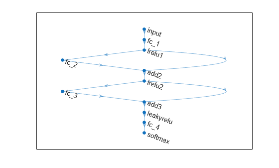
    Train a neural network classifier. Specify to have 35 outputs in the first fully connected layer and 20 outputs in the second fully connected layer. By default, both layers use a rectified linear unit (ReLU) activation function. You can change the activation functions for the fully connected layers by using the Activations name-value argument.

    Mdl = fitcnet(XTrain,YTrain, ...
        "LayerSizes",[35 20])
    Mdl = 
      ClassificationNeuralNetwork
                 ResponseName: 'Y'
        CategoricalPredictors: []
                   ClassNames: {'b'  'g'}
               ScoreTransform: 'none'
              NumObservations: 246
                   LayerSizes: [35 20]
                  Activations: 'relu'
        OutputLayerActivation: 'softmax'
                       Solver: 'LBFGS'
              ConvergenceInfo: [1x1 struct]
              TrainingHistory: [47x7 table]


    Access the weights and biases for the fully connected layers of the trained classifier by using the LayerWeights and LayerBiases properties of Mdl. The first two elements of each property correspond to the values for the first two fully connected layers, and the third element corresponds to the values for the final fully connected layer with a softmax activation function for classification. For example, display the weights and biases for the second fully connected layer.

    Mdl.LayerWeights{2}
    ans = 20×35
    
        0.0481    0.2501   -0.1535   -0.0934    0.0760   -0.0579   -0.2465    1.0411    0.3712   -1.2007    1.1162    0.4296    0.4045    0.5005    0.8839    0.4624   -0.3154    0.3454   -0.0487    0.2648    0.0732    0.5773    0.4286    0.0881    0.9468    0.2981    0.5534    1.0518   -0.0224    0.6894    0.5527    0.7045   -0.6124    0.2145   -0.0790
       -0.9489   -1.8343    0.5510   -0.5751   -0.8726    0.8815    0.0203   -1.6379    2.0315    1.7599   -1.4153   -1.4335   -1.1638   -0.1715    1.1439   -0.7661    1.1230   -1.1982   -0.5409   -0.5821   -0.0627   -0.7038   -0.0817   -1.5773   -1.4671    0.2053   -0.7931   -1.6201   -0.1737   -0.7762   -0.3063   -0.8771    1.5134   -0.4611   -0.0649
       -0.1910    0.0246   -0.3511    0.0097    0.3160   -0.0693    0.2270   -0.0783   -0.1626   -0.3478    0.2765    0.4179    0.0727   -0.0314   -0.1798   -0.0583    0.1375   -0.1876    0.2518    0.2137    0.1497    0.0395    0.2859   -0.0905    0.4325   -0.2012    0.0388   -0.1441   -0.1431   -0.0249   -0.2200    0.0860   -0.2076    0.0132    0.1737
       -0.0415   -0.0059   -0.0753   -0.1477   -0.1621   -0.1762    0.2164    0.1710   -0.0610   -0.1402    0.1452    0.2890    0.2872   -0.2616   -0.4204   -0.2831   -0.1901    0.0036    0.0781   -0.0826    0.1588   -0.2782    0.2510   -0.1069   -0.2692    0.2306    0.2521    0.0306    0.2524   -0.4218    0.2478    0.2343   -0.1031    0.1037    0.1598
        1.1848    1.6142   -0.1352    0.5774    0.5491    0.0103    0.0209    0.7219   -0.8643   -0.5578    1.3595    1.5385    1.0015    0.7416   -0.4342    0.2279    0.5667    1.1589    0.7100    0.1823    0.4171    0.7051    0.0794    1.3267    1.2659    0.3197    0.3947    0.3436   -0.1415    0.6607    1.0071    0.7726   -0.2840    0.8801    0.0848
        0.2486   -0.2920   -0.0004    0.2806    0.2987   -0.2709    0.1473   -0.2580   -0.0499   -0.0755    0.2000    0.1535   -0.0285   -0.0520   -0.2523   -0.2505   -0.0437   -0.2323    0.2023    0.2061   -0.1365    0.0744    0.0344   -0.2891    0.2341   -0.1556    0.1459    0.2533   -0.0583    0.0243   -0.2949   -0.1530    0.1546   -0.0340   -0.1562
       -0.0516    0.0640    0.1824   -0.0675   -0.2065   -0.0052   -0.1682   -0.1520    0.0060    0.0450    0.0813   -0.0234    0.0657    0.3219   -0.1871    0.0658   -0.2103    0.0060   -0.2831   -0.1811   -0.0988    0.2378   -0.0761    0.1714   -0.1596   -0.0011    0.0609    0.4003    0.3687   -0.2879    0.0910    0.0604   -0.2222   -0.2735   -0.1155
       -0.6192   -0.7804   -0.0506   -0.4205   -0.2584   -0.2020   -0.0008    0.0534    1.0185   -0.0307   -0.0539   -0.2020    0.0368   -0.1847    0.0886   -0.4086   -0.4648   -0.3785    0.1542   -0.5176   -0.3207    0.1893   -0.0313   -0.5297   -0.1261   -0.2749   -0.6152   -0.5914   -0.3089    0.2432   -0.3955   -0.1711    0.1710   -0.4477    0.0718
        0.5049   -0.1362   -0.2218    0.1637   -0.1282   -0.1008    0.1445    0.4527   -0.4887    0.0503    0.1453    0.1316   -0.3311   -0.1081   -0.7699    0.4062   -0.1105   -0.0855    0.0630   -0.1469   -0.2533    0.3976    0.0418    0.5294    0.3982    0.1027   -0.0973   -0.1282    0.2491    0.0425    0.0533    0.1578   -0.8403   -0.0535   -0.0048
        1.1109   -0.0466    0.4044    0.6366    0.1863    0.5660    0.2839    0.8793   -0.5497    0.0057    0.3468    0.0980    0.3364    0.4669    0.1466    0.7883   -0.1743    0.4444    0.4535    0.1521    0.7476    0.2246    0.4473    0.2829    0.8881    0.4666    0.6334    0.3105    0.9571    0.2808    0.6483    0.1180   -0.4558    1.2486    0.2453
          ⋮
    
    
    Mdl.LayerBiases{2}
    ans = 20×1
    
        0.6147
        0.1891
       -0.2767
       -0.2977
        1.3655
        0.0347
        0.1509
       -0.4839
       -0.3960
        0.9248
          ⋮


    The final fully connected layer has two outputs, one for each class in the response variable. The number of layer outputs corresponds to the first dimension of the layer weights and layer biases.

    size(Mdl.LayerWeights{end})
    ans = 1×2
    
         2    20
    
    
    size(Mdl.LayerBiases{end})
    ans = 1×2
    
         2     1


    To estimate the performance of the trained classifier, compute the test set classification error for Mdl.

    testError = loss(Mdl,XTest,YTest, ...
        "LossFun","classiferror")
    testError = 0.0774
    
    accuracy = 1 - testError
    accuracy = 0.9226
    

    Mdl accurately classifies approximately 92% of the observations in the test set.

    Extended Capabilities

    Version History

    Introduced in R2021a

    expand all