Main Content

refit

Class: FeatureSelectionNCAClassification

Refit neighborhood component analysis (NCA) model for classification

Syntax

mdlrefit = refit(mdl,Name,Value)

Description

mdlrefit = refit(mdl,Name,Value) refits the model mdl, with modified parameters specified by one or more Name,Value pair arguments.

Input Arguments

expand all

Neighborhood component analysis model or classification, specified as a FeatureSelectionNCAClassification object.

Name-Value Arguments

Specify optional pairs of arguments as Name1=Value1,...,NameN=ValueN, where Name is the argument name and Value is the corresponding value. Name-value arguments must appear after other arguments, but the order of the pairs does not matter.

Before R2021a, use commas to separate each name and value, and enclose Name in quotes.

Fitting Options

expand all

Method for fitting the model, specified as the comma-separated pair consisting of 'FitMethod' and one of the following.

  • 'exact' — Performs fitting using all of the data.

  • 'none' — No fitting. Use this option to evaluate the generalization error of the NCA model using the initial feature weights supplied in the call to fscnca.

  • 'average' — The function divides the data into partitions (subsets), fits each partition using the exact method, and returns the average of the feature weights. You can specify the number of partitions using the NumPartitions name-value pair argument.

Example: 'FitMethod','none'

Regularization parameter, specified as the comma-separated pair consisting of 'Lambda' and a non-negative scalar value.

For n observations, the best Lambda value that minimizes the generalization error of the NCA model is expected to be a multiple of 1/n

Example: 'Lambda',0.01

Data Types: double | single

Solver type for estimating feature weights, specified as the comma-separated pair consisting of 'Solver' and one of the following.

  • 'lbfgs' — Limited memory BFGS (Broyden-Fletcher-Goldfarb-Shanno) algorithm (LBFGS algorithm)

  • 'sgd' — Stochastic gradient descent

  • 'minibatch-lbfgs' — Stochastic gradient descent with LBFGS algorithm applied to mini-batches

Example: 'solver','minibatch-lbfgs'

Initial feature weights, specified as the comma-separated pair consisting of 'InitialFeatureWeights' and a p-by-1 vector of real positive scalar values.

Data Types: double | single

Indicator for verbosity level for the convergence summary display, specified as the comma-separated pair consisting of 'Verbose' and one of the following.

  • 0 — No convergence summary

  • 1 — Convergence summary including iteration number, norm of the gradient, and objective function value.

  • >1 — More convergence information depending on the fitting algorithm

    When using solver 'minibatch-lbfgs' and verbosity level >1, the convergence information includes iteration log from intermediate mini-batch LBFGS fits.

Example: 'Verbose',2

Data Types: double | single

LBFGS or Mini-Batch LBFGS Options

expand all

Relative convergence tolerance on the gradient norm for solver lbfgs, specified as the comma-separated pair consisting of 'GradientTolerance' and a positive real scalar value.

Example: 'GradientTolerance',0.00001

Data Types: double | single

SGD or Mini-Batch LBFGS Options

expand all

Initial learning rate for solver sgd, specified as the comma-separated pair consisting of 'InitialLearningRate' and a positive scalar value.

When using solver type 'sgd', the learning rate decays over iterations starting with the value specified for 'InitialLearningRate'.

Example: 'InitialLearningRate',0.8

Data Types: double | single

Maximum number of passes for solver 'sgd' (stochastic gradient descent), specified as the comma-separated pair consisting of 'PassLimit' and a positive integer. Every pass processes size(mdl.X,1) observations.

Example: 'PassLimit',10

Data Types: double | single

SGD or LBFGS or Mini-Batch LBFGS Options

expand all

Maximum number of iterations, specified as the comma-separated pair consisting of 'IterationLimit' and a positive integer.

Example: 'IterationLimit',250

Data Types: double | single

Output Arguments

expand all

Neighborhood component analysis model for classification, returned as a FeatureSelectionNCAClassification object. You can either save the results as a new model or update the existing model as mdl = refit(mdl,Name,Value).

Examples

expand all

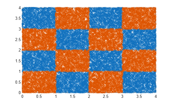
Generate checkerboard data using the generateCheckerBoardData.m function.

rng(2016,'twister'); % For reproducibility
pps = 1375;
[X,y] = generateCheckerBoardData(pps);
X = X + 2;

Plot the data.

figure
plot(X(y==1,1),X(y==1,2),'rx')
hold on
plot(X(y==-1,1),X(y==-1,2),'bx')

[n,p] = size(X)
n =

       22000


p =

     2

Add irrelevant predictors to the data.

Q = 98;
Xrnd = unifrnd(0,4,n,Q);
Xobs = [X,Xrnd];

This piece of code creates 98 additional predictors, all uniformly distributed between 0 and 4.

Partition the data into training and test sets. To create stratified partitions, so that each partition has similar proportion of classes, use y instead of length(y) as the partitioning criteria.

cvp = cvpartition(y,'holdout',2000);

cvpartition randomly chooses 2000 of the observations to add to the test set and the rest of the data to add to the training set. Create the training and validation sets using the assignments stored in the cvpartition object cvp .

Xtrain = Xobs(cvp.training(1),:);
ytrain = y(cvp.training(1),:);

Xval = Xobs(cvp.test(1),:);
yval = y(cvp.test(1),:);

Compute the misclassification error without feature selection.

nca = fscnca(Xtrain,ytrain,'FitMethod','none','Standardize',true, ...
    'Solver','lbfgs');
loss_nofs = loss(nca,Xval,yval)
loss_nofs =

    0.5165

'FitMethod','none' option uses the default weights (all 1s), which means all features are equally important.

This time, perform feature selection using neighborhood component analysis for classification, with $\lambda = 1/n$.

w0 = rand(100,1);
n = length(ytrain)
lambda = 1/n;
nca = refit(nca,'InitialFeatureWeights',w0,'FitMethod','exact', ...
       'Lambda',lambda,'solver','sgd');
n =

       20000

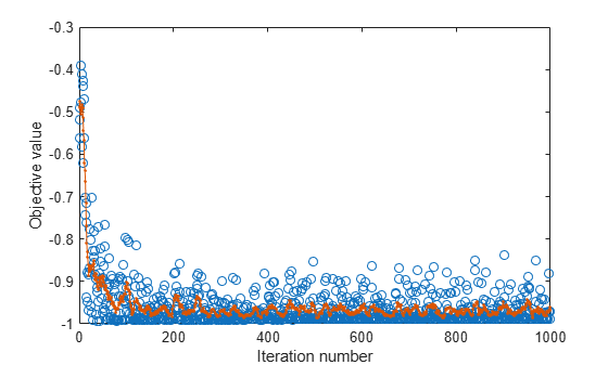
Plot the objective function value versus the iteration number.

figure()
plot(nca.FitInfo.Iteration,nca.FitInfo.Objective,'ro')
hold on
plot(nca.FitInfo.Iteration,movmean(nca.FitInfo.Objective,10),'k.-')
xlabel('Iteration number')
ylabel('Objective value')

Compute the misclassification error with feature selection.

loss_withfs = loss(nca,Xval,yval)
loss_withfs =

    0.0115

Plot the selected features.

figure
semilogx(nca.FeatureWeights,'ro')
xlabel('Feature index')
ylabel('Feature weight')
grid on

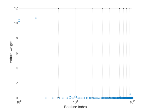
Select features using the feature weights and a relative threshold.

tol = 0.15;
selidx = find(nca.FeatureWeights > tol*max(1,max(nca.FeatureWeights)))
selidx =

     1
     2

Feature selection improves the results and fscnca detects the correct two features as relevant.

Version History

Introduced in R2016b