geocdf

Geometric cumulative distribution function

Syntax

y = geocdf(x,p)

y = geocdf(x,p,"upper")

Description

y = geocdf(x,p) returns the cumulative distribution function (cdf) of the geometric distribution, evaluated at each value in x using the corresponding probabilities in p.

y = geocdf(x,p,"upper") returns the complement of the cdf, evaluated at each value in x, using an algorithm that more accurately computes the extreme upper tail probabilities.

Examples

Compute Geometric Distribution cdf

Toss a fair coin repeatedly until the coin successfully lands with heads facing up. Determine the probability of observing at most three tails before tossing heads.

Compute the value of the cumulative distribution function (cdf) for the geometric distribution evaluated at the point x = 3, where x is the number of tails observed before the result is heads. Because the coin is fair, the probability of getting heads in any given toss is p = 0.5.

x = 3;
p = 0.5;
y = geocdf(x,p)

y = 
0.9375

The returned value y indicates that the probability of observing three or fewer tails before tossing heads is 0.9375.

Compute Multiple Geometric Distribution cdfs

Compare the cumulative distribution functions (cdfs) of three geometric distributions.

Create a probability vector that contains three different parameter values.

• The first parameter corresponds to a geometric distribution that models the number of times you toss a coin before the result is heads.

• The second parameter corresponds to a geometric distribution that models the number of times you roll a four-sided die before the result is a 4.

• The third parameter corresponds to a geometric distribution that models the number of times you roll a six-sided die before the result is a 6.

p = [1/2 1/4 1/6]'

p = 3×1

    0.5000
    0.2500
    0.1667

For each geometric distribution, evaluate the cdf at the points x = 0,1,2,...,25. Expand x and p so that the two geocdf input arguments have the same dimensions.

x = 0:25

x = 1×26

     0     1     2     3     4     5     6     7     8     9    10    11    12    13    14    15    16    17    18    19    20    21    22    23    24    25

expandedX = repmat(x,3,1);
expandedP = repmat(p,1,26);
y = geocdf(expandedX,expandedP)

y = 3×26

    0.5000    0.7500    0.8750    0.9375    0.9688    0.9844    0.9922    0.9961    0.9980    0.9990    0.9995    0.9998    0.9999    0.9999    1.0000    1.0000    1.0000    1.0000    1.0000    1.0000    1.0000    1.0000    1.0000    1.0000    1.0000    1.0000
    0.2500    0.4375    0.5781    0.6836    0.7627    0.8220    0.8665    0.8999    0.9249    0.9437    0.9578    0.9683    0.9762    0.9822    0.9866    0.9900    0.9925    0.9944    0.9958    0.9968    0.9976    0.9982    0.9987    0.9990    0.9992    0.9994
    0.1667    0.3056    0.4213    0.5177    0.5981    0.6651    0.7209    0.7674    0.8062    0.8385    0.8654    0.8878    0.9065    0.9221    0.9351    0.9459    0.9549    0.9624    0.9687    0.9739    0.9783    0.9819    0.9849    0.9874    0.9895    0.9913

Each row of y contains the cdf values for one of the three geometric distributions.

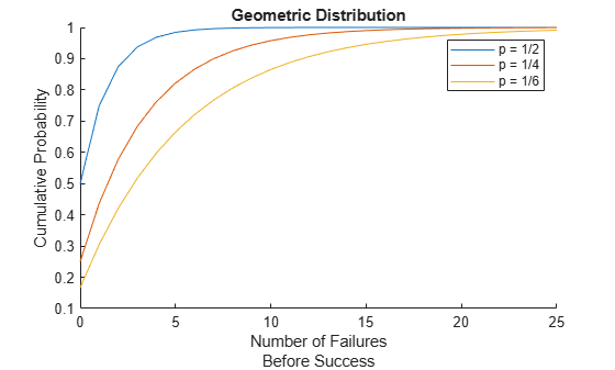
Compare the three geometric distributions by plotting the cdf values.

hold on
plot(x,y(1,:))
plot(x,y(2,:))
plot(x,y(3,:))
legend(["p = 1/2","p = 1/4","p = 1/6"])
xlabel(["Number of Failures","Before Success"])
ylabel("Cumulative Probability")
title("Geometric Distribution")
hold off

Compute Complement of Geometric Distribution cdf

Roll a fair die repeatedly until you successfully get a 6. Determine the probability of failing to roll a 6 within the first three rolls.

Compute the complement of the cumulative distribution function (cdf) for the geometric distribution evaluated at the point x = 2, where x is the number of non-6 rolls before the result is a 6. Note that an x value of 2 or less indicates successfully rolling a 6 within the first three rolls. Because the die is fair, the probability of getting a 6 in any given roll is p = 1/6.

x = 2;
p = 1/6;
y = geocdf(x,p,"upper")

y = 
0.5787

The returned value y indicates that the probability of failing to roll a 6 within the first three rolls is 0.5787. Note that this probability is equal to the probability of rolling a non-6 value three times.

probability = (1-p)^3

probability = 
0.5787

Input Arguments

x — Values at which to evaluate cdf

nonnegative integer scalar | array of nonnegative integer scalars

Values at which to evaluate the cdf, specified as a nonnegative integer scalar or an array of nonnegative integer scalars.

To evaluate the cdf at multiple values, specify x using an array. To evaluate the cdfs of multiple distributions, specify p using an array. If both of the input arguments x and p are arrays, then the array sizes must be the same. If only one of the input arguments is an array, then geocdf expands the scalar input into a constant array of the same size as the array input. Each element in y is the cdf value of the distribution specified by the corresponding element in p, evaluated at the corresponding element in x.

Example: 2

Example: [0 1 2 3]

Data Types: single | double

p — Probability of success

scalar in the range [0,1] | array of scalars in the range [0,1]

Probability of success in a single trial, specified as a scalar or an array of scalars in the range [0,1].

To evaluate the cdf at multiple values, specify x using an array. To evaluate the cdfs of multiple distributions, specify p using an array. If both of the input arguments x and p are arrays, then the array sizes must be the same. If only one of the input arguments is an array, then geocdf expands the scalar input into a constant array of the same size as the array input. Each element in y is the cdf value of the distribution specified by the corresponding element in p, evaluated at the corresponding element in x.

Example: 0.5

Example: [1/2 1/3]

Data Types: single | double

Output Arguments

y — cdf values

scalar in the range [0,1] | array of scalars in the range [0,1]

cdf values, returned as a scalar or an array of scalars in the range [0,1]. y is the same size as x and p after any necessary scalar expansion. For an element of y, y, and its corresponding elements in x and p, x and p, the cdf value y is the probability of having at most x trials before a success, when p is the probability of a success in any given trial.

More About

Geometric Distribution cdf

The geometric distribution is a one-parameter family of curves that models the number of failures before a success occurs in a series of independent trials. Each trial results in either success or failure, and the probability of success in any individual trial is constant. For example, if you toss a coin, the geometric distribution models the number of tails observed before the result is heads. The geometric distribution is discrete, existing only on the nonnegative integers.

The cumulative distribution function (cdf) of the geometric distribution is

$$y=F(x|p)=1-{\left(1-p\right)}^{x+1};x=0,1,2,\mathrm{...},$$

where p is the probability of success, and x is the number of failures before the first success. The result y is the probability of observing up to x trials before a success, when the probability of success in any given trial is p.

References

[1] Abramowitz, M., and I. A. Stegun. Handbook of Mathematical Functions. New York: Dover, 1964.

[2] Evans, M., N. Hastings, and B. Peacock. Statistical Distributions. 2nd ed., Hoboken, NJ: John Wiley & Sons, Inc., 1993.

Extended Capabilities

C/C++ Code Generation
Generate C and C++ code using MATLAB® Coder™.

GPU Arrays

Accelerate code by running on a graphics processing unit (GPU) using Parallel Computing Toolbox™.

This function fully supports GPU arrays. For more information, see Run MATLAB Functions on a GPU (Parallel Computing Toolbox).

Version History

Introduced before R2006a