Main Content

wt

Continuous wavelet transform with filter bank

Description

example

cfs = wt(fb,x) returns the continuous wavelet transform (CWT) coefficients of the signal x, using fb, a CWT filter bank. x is a real- or complex-valued vector. x must have at least 4 samples. If x is real-valued, cfs is a 2-D matrix, where each row corresponds to one scale. The column size of cfs is equal to the length of x. If x is complex-valued, cfs is a 3-D array, where the first page is the CWT for the positive scales (analytic part or counterclockwise component), and the second page is the cwt for the negative scales (anti-analytic part or clockwise component).

[cfs,f] = wt(fb,x) returns the frequencies f corresponding to the scales (rows) of cfs if the SamplingPeriod property is not specified in the CWT filter bank fb. If you do not specify a sampling frequency, f is in cycles/sample.

[cfs,f,coi] = wt(fb,x) returns the cone of influence coi for the CWT. coi is in the same units as f. If the input x is complex, the coi applies to both pages of cfs.

example

[cfs,f,coi,scalcfs] = wt(fb,x) returns the scaling coefficients scalcfs for the wavelet transform.

[cfs,p] = wt(fb,x) returns the periods p corresponding to the scales (rows) of cfs if you specify a sampling period in the CWT filter bank. p has the same units and format as the duration scalar sampling period.

[cfs,p,coi] = wt(fb,x) returns the cone of influence coi in periods for the CWT. coi is an array of durations with the same format property as the sampling period. If the input x is complex, the coi applies to both pages of cfs.

[cfs,p,coi,scalcfs] = wt(fb,x) returns the scaling coefficients scalcfs for the wavelet transform.

Examples

collapse all

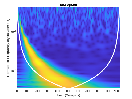
Load the noisy Doppler signal. Create a CWT filter bank that can be applied to the signal.

load noisdopp
fb = cwtfilterbank('SignalLength',numel(noisdopp));

Use the filter bank to obtain the continuous wavelet transform of the signal.

[cfs,f,coi] = wt(fb,noisdopp);

Plot the CWT scalogram, including the cone of influence.

t = 0:numel(noisdopp)-1;
pcolor(t,f,abs(cfs))
shading flat
set(gca,'YScale','log')
hold on
plot(t,coi,'w-','LineWidth',3)
xlabel('Time (Samples)')
ylabel('Normalized Frequency (cycles/sample)')
title('Scalogram')

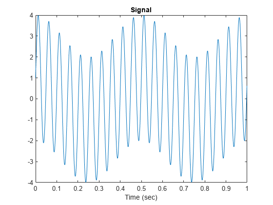
Create and plot a signal sampled at 1000 Hz. Create a CWT filter bank that can be used on the signal. Since the signal is periodic, set the boundary extension property of the filter bank to 'periodic'.

Fs = 1000;
t = 0:1/Fs:1-1/Fs;
sig = 3*sin(2*pi*20*t) + cos(2*pi*2*t);
fb = cwtfilterbank('SignalLength',length(sig),...
    'SamplingFrequency',Fs,...
    'Boundary','periodic');
plot(t,sig)
xlabel('Time (sec)')
title('Signal')

Take the CWT of the signal. Return the wavelet and scaling coefficients.

[cfs,~,~,scalcfs] = wt(fb,sig);

Reconstruct the signal two ways. First use the mean of the signal, then use the scaling coefficients. Plot the difference between the original signal and both reconstructions.

xrec0 = icwt(cfs,'SignalMean',mean(sig));
xrec1 = icwt(cfs,'ScalingCoefficients',scalcfs);
plot(t,sig-xrec0)
hold on
plot(t,sig-xrec1)
grid on
legend('Using mean(sig)','Using scalcfs')
title('Difference Between Reconstructions')

The scaling coefficients results in a significantly more accurate reconstruction. To investigate the source of the dramatic improvement, create a second signal consisting of the 2 Hz component of the original signal. Compare the scaling coefficients with the 2 Hz signal. The scaling coefficients and 2 Hz signal are virtually identical. Using the scaling coefficients helps with the reconstruction because the 2 Hz component is not representable by a wavelet with this sampling frequency and length.

figure
sig2hz = cos(2*pi*2*t);
plot(t,sig2hz)
hold on
plot(t,scalcfs)
grid on
title('Comparing Scaling Coefficients with 2 Hz Component')
xlabel('Time (sec)')
legend('2 Hz Component', 'Scaling Coefficients')

This example shows how using a CWT filter bank can improve computational efficiency when taking the CWT of multiple time series.

Create a 100-by-1024 matrix x. Create a CWT filter bank appropriate for signals with 1024 samples.

x = randn(100,1024);
fb = cwtfilterbank;

Use cwt with default settings to obtain the CWT of a signal with 1024 samples. Create a 3-D array that can contain the CWT coefficients of 100 signals, each of which has 1024 samples.

cfs = cwt(x(1,:));
res = zeros(100,size(cfs,1),size(cfs,2));

Use the cwt function and take the CWT of each row of the matrix x. Display the elapsed time.

tic
for k=1:100
    res(k,:,:) = cwt(x(k,:));
end
toc
Elapsed time is 0.928160 seconds.

Now use the wt object function of the filter bank to take the CWT of each row of x. Display the elapsed time.

tic
for k=1:100
    res(k,:,:) = wt(fb,x(k,:));
end
toc
Elapsed time is 0.393524 seconds.

Input Arguments

collapse all

Continuous wavelet transform (CWT) filter bank, specified as a cwtfilterbank object.

Input signal, specified as a real- or complex-valued vector. x must have at least four samples.

Data Types: double | single
Complex Number Support: Yes

Output Arguments

collapse all

Continuous wavelet transform, returned as a matrix or 3-D array of complex values. If x is real-valued, cfs is a 2-D matrix, where each row corresponds to one scale. The column size of cfs is equal to the length of x. If x is complex-valued, cfs is a 3-D array, where the first page is the CWT for the positive scales (analytic part or counterclockwise component), and the second page is the CWT for the negative scales (anti-analytic part or clockwise component).

Data Types: double | single

Frequencies, returned as a vector, corresponding to the scales (rows) of cfs if the 'SamplingPeriod' is not specified in fb. If you specify a sampling frequency, f is in hertz. If you do not specify a frequency, f is in cycles/sample.

Data Types: double

Periods, returned as an array of durations, corresponding to the scales (rows) of cfs if fb has a specified sampling period. p has the same units and format as the duration scalar sampling period.

Data Types: duration

Cone of influence for the CWT, returned as either an array of real numbers or an array of durations. The cone of influence indicates where edge effects occur in the CWT. If you specify a sampling frequency, coi is an array of real numbers in the same units as f. If you specify a sampling period, coi is an array of durations with the same format property as the sampling period. Due to the edge effects, give less credence to areas that are outside or overlap the cone of influence.

For additional information, see Boundary Effects and the Cone of Influence.

Data Types: double | duration

Scaling coefficients for the wavelet transform, returned as a vector with the same length as x. If x is real-valued, scalcfs is real valued. If x is complex-valued, scalcfs is complex-valued.

Data Types: double

Tips

  • The first time you use a filter bank to take the CWT of a signal, the wavelet filters are constructed to have the same datatype as the signal. A warning message is generated when you apply the same filter bank to a signal with a different datatype. Changing datatypes comes with the cost of redesigning or changing the precision of the filter bank. For optimal performance, use a consistent datatype.

  • When performing multiple CWTs, for example inside a for-loop, the recommended workflow is to first create a cwtfilterbank object and then use the wt object function. This workflow minimizes overhead and maximizes performance. See Using CWT Filter Bank on Multiple Time Series.
Extended Capabilities

C/C++ Code Generation
Generate C and C++ code using MATLAB® Coder™.

Version History

Introduced in R2018a