FFT with normalized spatial frequency for image sensor MTF

I'm attempting to use the slanted edge method to calculate the MTF for a camera system according to Harvest Imaging (https://harvestimaging.com/blog/?p=1328), and struggling to plot the result correctly. The method involves taking the Fourier transform of a line spread function and plotting it from DC to the sampling frequency. I have chosen the sampling frequency to equal 2, since that is the minimum number of pixels required to record contrast. Here is my code:

LSF = [];
LSF(1:250) = 0;
LSF(51:70) = 140;

Fs = 2;             % Sampling frequency   (pixels/lp)                 
T = 1/Fs;           % Sampling period     (lp/pixel) 
L = length(LSF);    % Length of signal    (length of line in pixels)

P2 = abs(fft(LSF/L));
P1 = P2(1:L/2+1);
P1(2:end-1) = 2*P1(2:end-1);

f = Fs*(0:(L/2))/L;
nP1 = P1-min(P1);
nP1 = nP1./max(nP1);
plot(f,nP1,'linewidth',3) 
title('MTF')
xlabel('Normalized Spatial Frequency')

According to the example, I should reach my first minimum of the sinc function at x=1

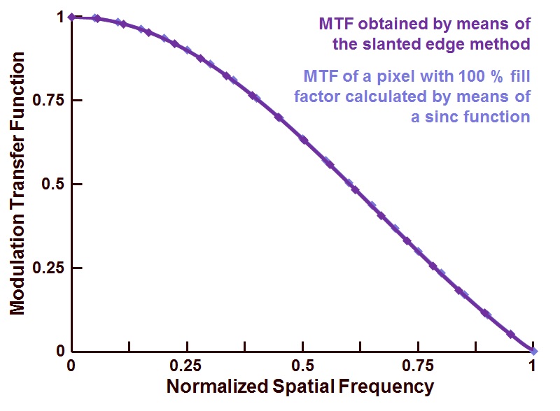
But, I appear to be off by a factor of 10.

Can anyone point out where I'm going wrong? I'm sure it's a simple fix.

Thanks much!

[David Goodmanson]

Hello Ben,

No comment on the interpretation, but a width-two pulse is the only one whose fft is a sinc-like function with its first zero at the edges of the resulting frequency array.

[Ben Hendrickson]

Thanks David,

That makes sense, but I'm trying to reproduce the curves as seen in the tutorial I included in the post. Changing the width of the rectangular pulse seems like cheating.

Ben

[David Goodmanson]

Hello Ben,

I could have been clearer in the comment so I modified it.

[Ben Hendrickson]

Hey David,

Appreciate the clarification. I’m curious how the author of the tutorial got that result from this LSF:

Am I misinterpreting the sampling frequency somehow? He gave an example of using Fs=200, which stems from assuming a 5 micron pixel pitch -> 200 line pairs per millimeter at the sampling frequency (a standard unit when measuring MTF, i.e. 200 lap/mm = 1 normalized spatial frequency)

I understand your not the author of the tutorial, but if you have a guess I’m all ears. It’s as good as mine!

[David Goodmanson]

Hello Ben, see these two for a clearer explanation of the method.

https://www.strollswithmydog.com/the-slanted-edge-method/

http://www.strollswithmydog.com/units-spatial-resolution/

The Harvest blog calls the original function (before taking a derivative) the 'spectral frequency response' which I think is confusing if not incorrect. Certainly the idea is to fourier transform a 1d point spread function in pixels to obtain the modulation transfer function in cycles / pixel. Knowing pixel pitch produces cycles per mm. Then a factor of 1/2 to get line pairs / mm ?

[Ben Hendrickson]

Appreciate the links! I agree that it should be obtained in cycles/pixel, then coverted to lp/mm. The problem may have to do with the say the initial function (SFR) is plotted. The idea is to super-resolve the edge, which means it should be plotted against fractions of a pixel. Mine is not. I'll keep banging my head against it and let you know when I've figured it out.

Thanks for talking it out with me!

[Ali Madani]

Hi Ben, did you figure out how to normalized the x-axis? I've been having the same question and cannot figure out how to do this.

Answer 1

[Jack]

Hi Ben,

You are off by a factor of 10 because there are 10 samples in one of your 'pixels'. The result of the FT is in cycles/set, which can also be expressed in other units as shown below (see here for a detailed explanation). I used similar figures to yours that however result in the sinc having samples at MTF nulls.

Jack

n = 256;                                %samples per set
px = 16;                                %samples per pixel
LSF = zeros(1,n);                 
LSF(1:px)=140;                          %the pixel has intensity 140

MTF = 1/sum(LSF) * abs(fft(LSF));   
f = 0:n-1;                              %cycles per set

figure; plot(f,MTF);                    %cycles per set
xlabel('cycles/set'); ylabel('MTF')
figure; plot(f/n,MTF);                  %cycles per sample
xlabel('cycles/sample'); ylabel('MTF')
figure; plot (f/n*px,MTF)               %cycles per pixel
xlabel('cycles/pixel'); ylabel('MTF'); xlim([0 1])