Résultats pour
Automating Parameter Identifiability Analysis in SimBiology
Is it possible to develop a MATLAB Live Script that automates a series of SimBiology model fits to obtain likelihood profiles? The goal is to fit a kinetic model to experimental data while systematically fixing the value of one kinetic constant (e.g., k1) and leaving the others unrestricted.
The script would perform the following:
Use a pre-configured SimBiology project where the best fit to the experimental data has already been established (including dependent/independent variables, covariates, the error model, and optimization settings).
Iterate over a defined sequence of fixed values for a chosen parameter.
For each fixed value, run the estimation to optimize the remaining parameters.
Record the resulting Sum of Squared Errors (SSE) for each run.
The final output would be a likelihood profile—a plot of SSE versus the fixed parameter value (e.g., k1)—to assess the practical identifiability of each model parameter.
For the www, uk, and in domains,a generative search answer is available for Help Center searches. Please let us know if you get good or bad results for your searches. Some have pointed out that it is not available in non-english domains. You can switch your country setting to try it out. You can also ask questions in different languages and ask for the response in a different language. I get better results when I ask more specific queries. How is it working for you?
Hello MATLAB Central community,
My name is Yann. And I love MATLAB. I also love Python ... 🐍 (I know, not the place for that).
I recently decided to go down the rabbit hole of AI. So I started benchmarking deep learning frameworks on basic examples. Here is a recording of my experiment:
Happy to engage in the debate. What do you think?
Large Language Models (LLMs) with MATLAB was updated again today to support the newly released OpenAI models GPT-5, GPT-5 mini, GPT-5 nano, GPT-5 chat, o3, and o4-mini. When you create an openAIChat object, set the ModelName name-value argument to "gpt-5", "gpt-5-mini", "gpt-5-nano", "gpt-5-chat-latest", "o4-mini", or "o3".
This is version 4.4.0 of this free MATLAB add-on that lets you interact with LLMs on MATLAB. The release notes are at Release v4.4.0: Support for GPT-5, o3, o4-mini · matlab-deep-learning/llms-with-matlab
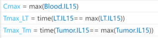
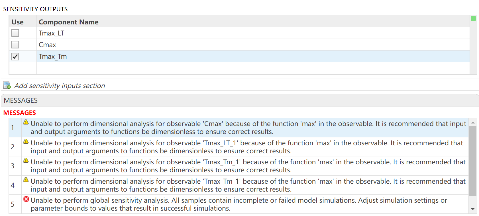
I want to observe the time (Tmax) to reach maximum drug concentration (Cmax) in my model. I have set up the OBSERVABLES as follows (figure1): Cmax = max(Blood.lL15); Tmax_LT = time(Conc_lL15_LT_nm == max(Conc_lL15_LT_nm)); Tmax_Tm = time(Conc_lL15_Tumor_nm == max(Conc_lL15_Tumor_nm)); After running the Sobol indices program for global sensitivity analysis, with inputs being some parameters and their ranges, the output for Cmax works, but there are some prompts, as shown in figure2. Additionally, when outputting Tmax, the program does not run successfully and reports some errors, as shown in figure2. How can I resolve the errors when outputting Tmax?
Large Languge model with MATLAB, a free add-on that lets you access LLMs from OpenAI, Azure, amd Ollama (to use local models) on MATLAB, has been updated to support OpenAI GPT-4.1, GPT-4.1 mini, and GPT-4.1 nano.
According to OpenAI, "These models outperform GPT‑4o and GPT‑4o mini across the board, with major gains in coding and instruction following. They also have larger context windows—supporting up to 1 million tokens of context—and are able to better use that context with improved long-context comprehension."
What would you build with the latest update?

Provide insightful answers
9%
Provide label-AI answer
9%
Provide answer by both AI and human
21%
Do not use AI for answers
46%
Give a button "chat with copilot"
10%
use AI to draft better qustions
5%
1561 votes
%% 清理环境
close all; clear; clc;
%% 模拟时间序列
t = linspace(0,12,200); % 时间从 0 到 12,分 200 个点
% 下面构造一些模拟的"峰状"数据,用于演示
% 你可以根据需要替换成自己的真实数据
rng(0); % 固定随机种子,方便复现
baseIntensity = -20; % 强度基线(z 轴的最低值)
numSamples = 5; % 样本数量
yOffsets = linspace(20,140,numSamples); % 不同样本在 y 轴上的偏移
colors = [ ...
0.8 0.2 0.2; % 红
0.2 0.8 0.2; % 绿
0.2 0.2 0.8; % 蓝
0.9 0.7 0.2; % 金黄
0.6 0.4 0.7]; % 紫
% 构造一些带多个峰的模拟数据
dataMatrix = zeros(numSamples, length(t));
for i = 1:numSamples
% 随机峰参数
peakPositions = randperm(length(t),3); % 三个峰位置
intensities = zeros(size(t));
for pk = 1:3
center = peakPositions(pk);
width = 10 + 10*rand; % 峰宽
height = 100 + 50*rand; % 峰高
% 高斯峰
intensities = intensities + height*exp(-((1:length(t))-center).^2/(2*width^2));
end
% 再加一些小随机扰动
intensities = intensities + 10*randn(size(t));
dataMatrix(i,:) = intensities;
end
%% 开始绘图
figure('Color','w','Position',[100 100 800 600],'Theme','light');
hold on; box on; grid on;
for i = 1:numSamples
% 构造 fill3 的多边形顶点
xPatch = [t, fliplr(t)];
yPatch = [yOffsets(i)*ones(size(t)), fliplr(yOffsets(i)*ones(size(t)))];
zPatch = [dataMatrix(i,:), baseIntensity*ones(size(t))];
% 使用 fill3 填充面积
hFill = fill3(xPatch, yPatch, zPatch, colors(i,:));
set(hFill,'FaceAlpha',0.8,'EdgeColor','none'); % 调整透明度、去除边框
% 在每条曲线尾部标注 Sample i
text(t(end)+0.3, yOffsets(i), dataMatrix(i,end), ...
['Sample ' num2str(i)], 'FontSize',10, ...
'HorizontalAlignment','left','VerticalAlignment','middle');
end
%% 坐标轴与视角设置
xlim([0 12]);
ylim([0 160]);
zlim([-20 350]);
xlabel('Time (sec)','FontWeight','bold');
ylabel('Frequency (Hz)','FontWeight','bold');
zlabel('Intensity','FontWeight','bold');
% 设置刻度(根据需要微调)
set(gca,'XTick',0:2:12, ...
'YTick',0:40:160, ...
'ZTick',-20:40:200);
% 设置视角(az = 水平旋转,el = 垂直旋转)
view([211 21]);
% 让三维坐标轴在后方
set(gca,'Projection','perspective');
% 如果想去掉默认的坐标轴线,也可以尝试
% set(gca,'BoxStyle','full','LineWidth',1.2);
%% 可选:在后方添加一个浅色网格平面 (示例)
% 这个与题图右上方的网格类似
[Xplane,Yplane] = meshgrid([0 12],[0 160]);
Zplane = baseIntensity*ones(size(Xplane)); % 在 Z = -20 处画一个竖直面的框
surf(Xplane, Yplane, Zplane, ...
'FaceColor',[0.95 0.95 0.9], ...
'EdgeColor','k','FaceAlpha',0.3);
%% 进一步美化(可根据需求调整)
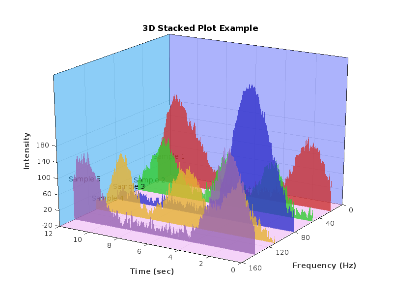
title('3D Stacked Plot Example','FontSize',12);
constantplane("x",12,FaceColor=rand(1,3),FaceAlpha=0.5);
constantplane("y",0,FaceColor=rand(1,3),FaceAlpha=0.5);
constantplane("z",-19,FaceColor=rand(1,3),FaceAlpha=0.5);
hold off;
Have fun! Enjoy yourself!
We are excited to announce the first edition of the MathWorks AI Challenge. You’re invited to submit innovative solutions to challenges in the field of artificial intelligence. Choose a project from our curated list and submit your solution for a chance to win up to $1,000 (USD). Showcase your creativity and contribute to the advancement of AI technology.
Simulink has been an essential tool for modeling and simulating dynamic systems in MATLAB. With the continuous advancements in AI, automation, and real-time simulation, I’m curious about what the future holds for Simulink.
What improvements or new features do you think Simulink will have in the coming years? Will AI-driven modeling, cloud-based simulation, or improved hardware integration shape the next generation of Simulink?
You've probably heard about the DeepSeek AI models by now. Did you know you can run them on your own machine (assuming its powerful enough) and interact with them on MATLAB?
In my latest blog post, I install and run one of the smaller models and start playing with it using MATLAB.
Larger models wouldn't be any different to use assuming you have a big enough machine...and for the largest models you'll need a HUGE machine!
Even tiny models, like the 1.5 billion parameter one I demonstrate in the blog post, can be used to demonstrate and teach things about LLM-based technologies.
Have a play. Let me know what you think.
Is it possible to differenciate the input, output and in-between wires by colors?
I was curious to startup your new AI Chat playground.
The first screen that popped up made the statement:
"Please keep in mind that AI sometimes writes code and text that seems accurate, but isnt"
Can someone elaborate on what exactly this means with respect to your AI Chat playground integration with the Matlab tools?
Are there any accuracy metrics for this integration?
Watch episodes 5-7 for the new stuff, but the whole series is really great.
Local large language models (LLMs), such as llama, phi3, and mistral, are now available in the Large Language Models (LLMs) with MATLAB repository through Ollama™!
Read about it here:
Hi All,
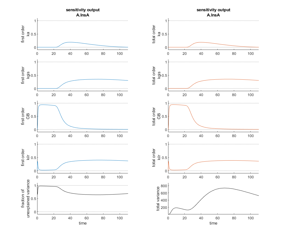
I'm currently verifying a global sensitivity analysis done in SimBiology and I'm a touch confused. This analysis was run with every parameter and compartment volume in the model. To my understanding the fraction of unexplained variance is 1 - the sum of the first order variances, therefore if the model dynamics are dominated by interparameter effects you might see a higher fraction of unexplained variance. In this analysis however, as the attached figure shows (with input at t=20 minutes), the most sensitive four parameters seem to sum, in first order sensitivities to roughly one at each time point and the total order sensitivies appear nearly identical. So how is the fraction of unexplained variance near one?
Thank you for your help!
hello i found the following tools helpful to write matlab programs. copilot.microsoft.com chatgpt.com/gpts gemini.google.com and ai.meta.com. thanks a lot and best wishes.
Check out the LLMs with MATLAB project on File Exchange to access Large Language Models from MATLAB.
Along with the latest support for GPT-4o mini, you can use LLMs with MATLAB to generate images, categorize data, and provide semantic analyis.
What do you think about the NVIDIA's achivement of becoming the top giant of manufacturing chips, especially for AI world?

Hi to everyone!
To simplify the explanation and the problem, I simulated the kinetics of an irreversible first-order reaction, A -> B. I implemented it in two independent compartments, R and P. I simulated the effect of a dilution in R by doubling at t= 0,1 the R volume. I programmed in P that, at t = 0.1, the instantaneous concentration of A and B would be reduced by half. I am sending an attach with the implementation of these simulations in the Simbiology interface.
When the simulations of the two compartments are plotted, it can be seen that the responses are not equal. That is, from t = 0.1 s, the reaction follow an exponential function in R with half of the initial amplitude and half of the initial value of k1. That is, the relaxation time is doubled. Meanwhile, in P, from t = 0.1, the reaction follows exponential kinetics with half the amplitude value but maintaining the initial value of k = 10. Without a doubt, the correct simulation is the latter (compartment P) where only the effect is observed in the amplitude and not in the relaxation time. Could you tell me what the error is that makes these kinetics that should be equal not be?
Thank you in advance!
Luis B.