Base case:
Suppose you need to do a computation many times. We are going to assume that this computation cannot be vectorized. The simplest case is to use a for loop:
number_of_elements = 1e6;
test_fcn = @(x) sqrt(x) / x;
tic
for i = 1:number_of_elements
x(i) = test_fcn(i);
end
t_forward = toc;
disp(t_forward + " seconds")
Preallocation:
This can easily be sped up by preallocating the variable that houses results:
tic
x = zeros(number_of_elements, 1);
for i = 1:number_of_elements
x(i) = test_fcn(i);
end
t_forward_prealloc = toc;
disp(t_forward_prealloc + " seconds")
In this example, preallocation speeds up the loop by a factor of about three to four (running in R2024a). Comment below if you get dramatically different results.
disp(sprintf("%.1f", t_forward / t_forward_prealloc))
Run it in reverse:
Is there a way to skip the explicit preallocation and still be fast? Indeed, there is.
clear x
tic
for i = number_of_elements:-1:1
x(i) = test_fcn(i);
end
t_backward = toc;
disp(t_backward + " seconds")
By running the loop backwards, the preallocation is implicitly performed during the first iteration and the loop runs in about the same time (within statistical noise):
disp(sprintf("%.2f", t_forward_prealloc / t_backward))
Do you get similar results when running this code? Let us know your thoughts in the comments below.
Beneficial side effect:
Have you ever had to use a for loop to delete elements from a vector? If so, keeping track of index offsets can be tricky, as deleting any element shifts all those that come after. By running the for loop in reverse, you don't need to worry about index offsets while deleting elements.
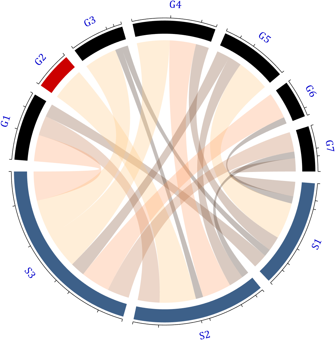
Chord diagrams are very common in Python and R, but there are no related functions in MATLAB before. It is not easy to draw chord diagrams of the same quality as R language, But I created a MATLAB tool that could almost do it.
↓ ↓ ↓ ↓ ↓ ↓ ↓ ↓ ↓ ↓
↑ ↑ ↑ ↑ ↑ ↑ ↑ ↑ ↑ ↑
Here is the help document:
1 Data Format
The data requirement is a numerical matrix with all values greater than or equal to 0, or a table array, or a numerical matrix and cell array for names. First, give an example of a numerical matrix:
1.1 Numerical Matrix
dataMat=randi([0,5],[5,4]);
% 绘图(draw)
CC=chordChart(dataMat);
CC=CC.draw();
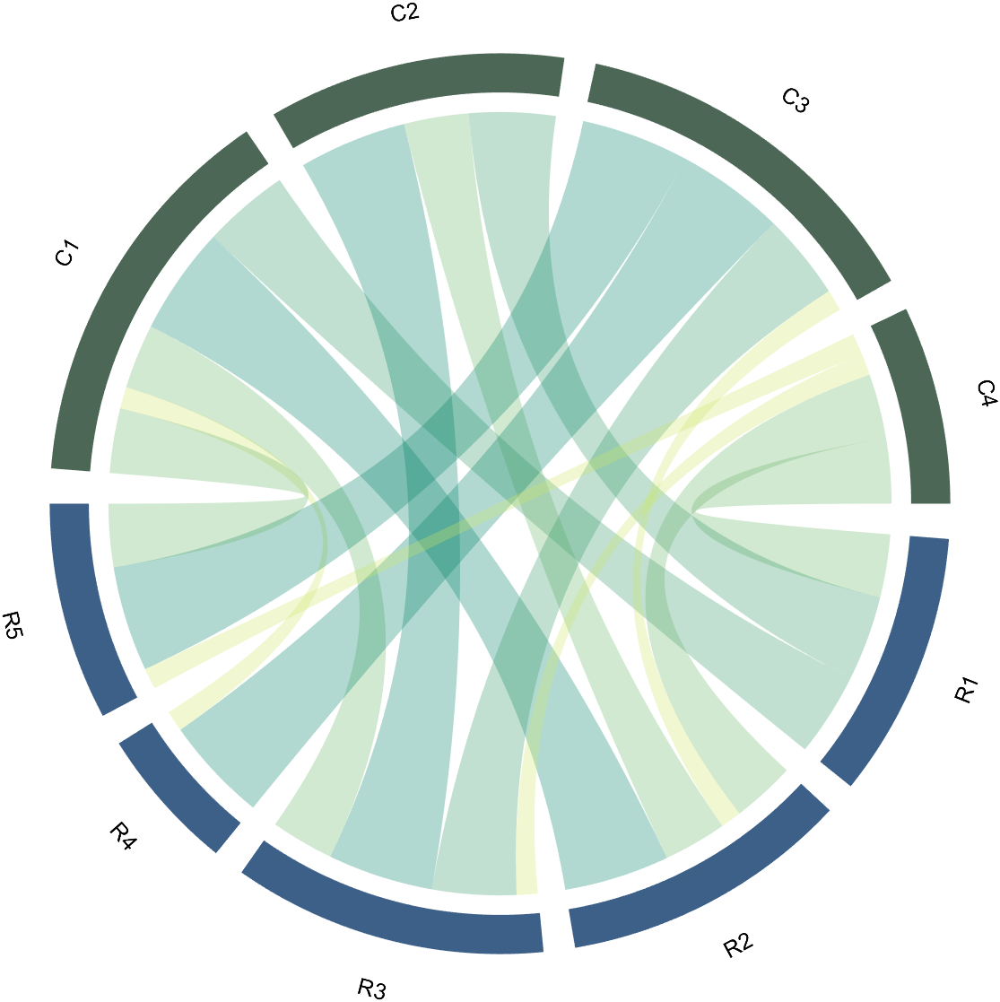
Since each object is not named, it will be automatically named Rn and Cn
1.2 Numerical Matrix and Cell Array for Names
dataMat=[2 0 1 2 5 1 2;
3 5 1 4 2 0 1;
4 0 5 5 2 4 3];
colName={'G1','G2','G3','G4','G5','G6','G7'};
rowName={'S1','S2','S3'};
CC=chordChart(dataMat,'rowName',rowName,'colName',colName);
CC=CC.draw();

RowName should be the same size as the rows of the matrix
ColName should be the same size as the columns of the matrix
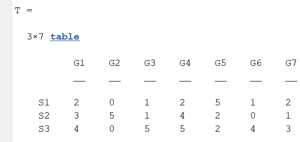
For this example, if the value in the second row and third column is 1, it indicates that there is an energy flow from S2 to G3, and a chord with a width of 1 is needed between these two.
1.3 Table Array
A table array in the following format is required:
2 Decorate Chord
2.1 Batch modification of chords
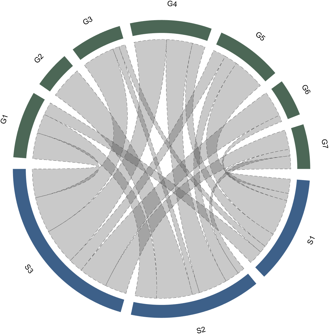
Batch modification of chords can be done using the setChordProp function, and all properties of the Patch object can be modified. For example, modifying the color of the string, edge color, edge line sstyle, etc.:
CC.setChordProp('EdgeColor',[.3,.3,.3],'LineStyle','--',...
'LineWidth',.1,'FaceColor',[.3,.3,.3])
2.2 Individual Modification of Chord
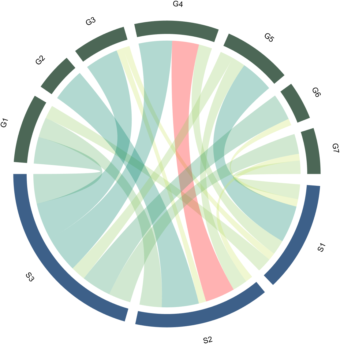
The individual modification of chord can be done using the setChordMN function, where the values of m and n correspond exactly to the rows and columns of the original numerical matrix. For example, changing the color of the strings flowing from S2 to G4 to red:
CC.setChordMN(2,4,'FaceColor',[1,0,0])
2.3 Color Mapping of Chords
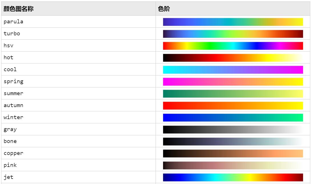
Just use function colormap to do so:
% version 1.7.0更新
% 可使用colormap函数直接修改颜色
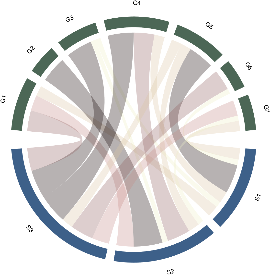
% Colors can be adjusted directly using the function colormap(demo4)
colormap(flipud(pink))
3 Arc Shaped Block Decoration
3.1 Batch Decoration of Arc-Shaped Blocks
use:
- setSquareT_Prop
- setSquareF_Prop
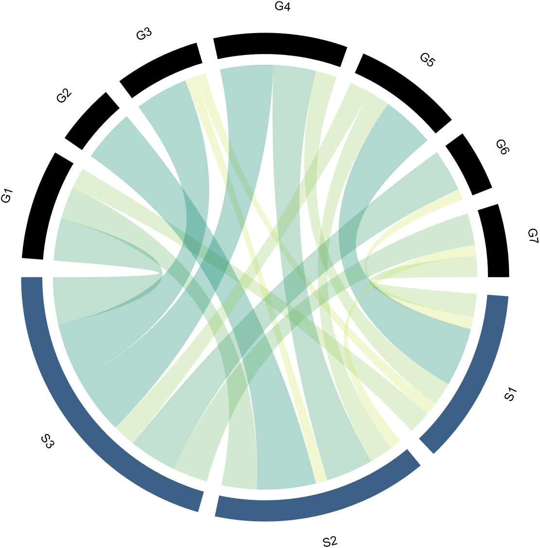
to modify the upper and lower blocks separately, and all attributes of the Patch object can be modified. For example, batch modify the upper blocks (change to black):
CC.setSquareT_Prop('FaceColor',[0,0,0])
3.2 Arc-Shaped Blocks Individually Decoration
use:
- setSquareT_N
- setSquareF_N
to modify the upper and lower blocks separately. For example, modify the second block above separately (changed to red):
CC.setSquareT_N(2,'FaceColor',[.8,0,0])
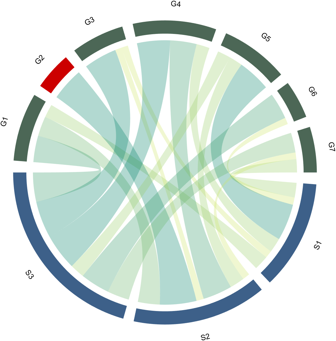
4 Font Adjustment
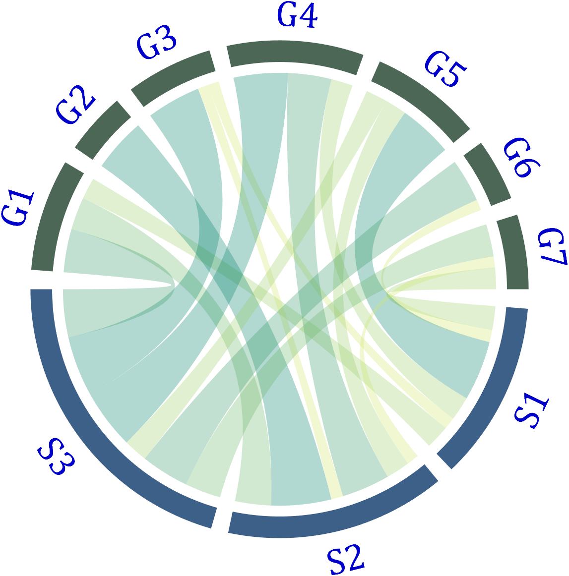
Use the setFont function to adjust the font, and all properties of the text object can be modified. For example, changing the font size, font, and color of the text:
CC.setFont('FontSize',25,'FontName','Cambria','Color',[0,0,.8])
5 Show and Hide Ticks
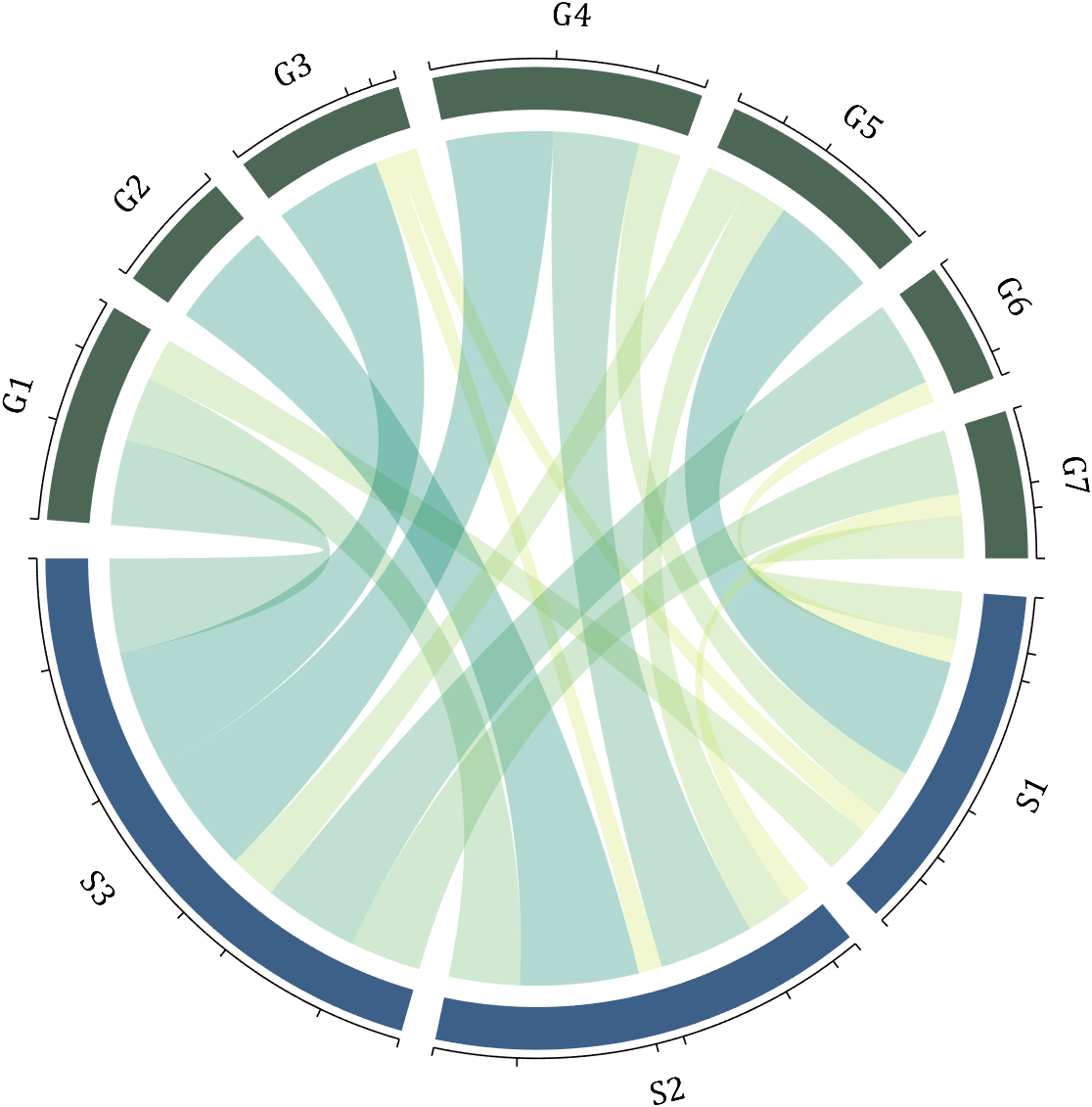
Usage:
CC.tickState('on')
% CC.tickState('off')
6 Attribute 'Sep' with Adjustable Square Spacing
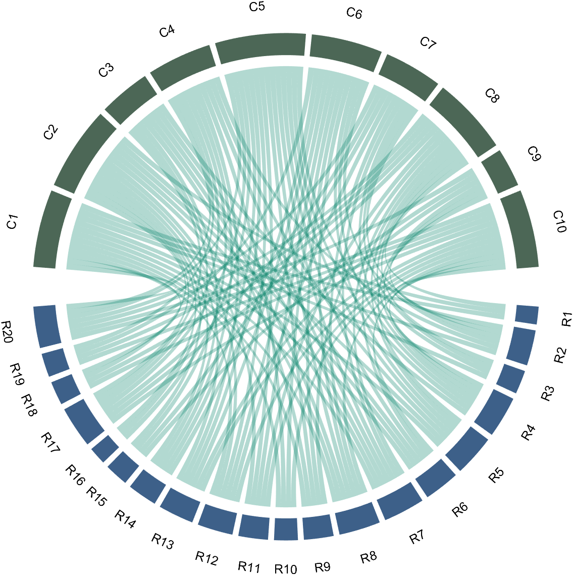
If the matrix size is large, the drawing will be out of scale:
dataMat=randi([0,1],[20,10]);
CC=chordChart(dataMat);
CC=CC.draw();
% CC.tickState('on')
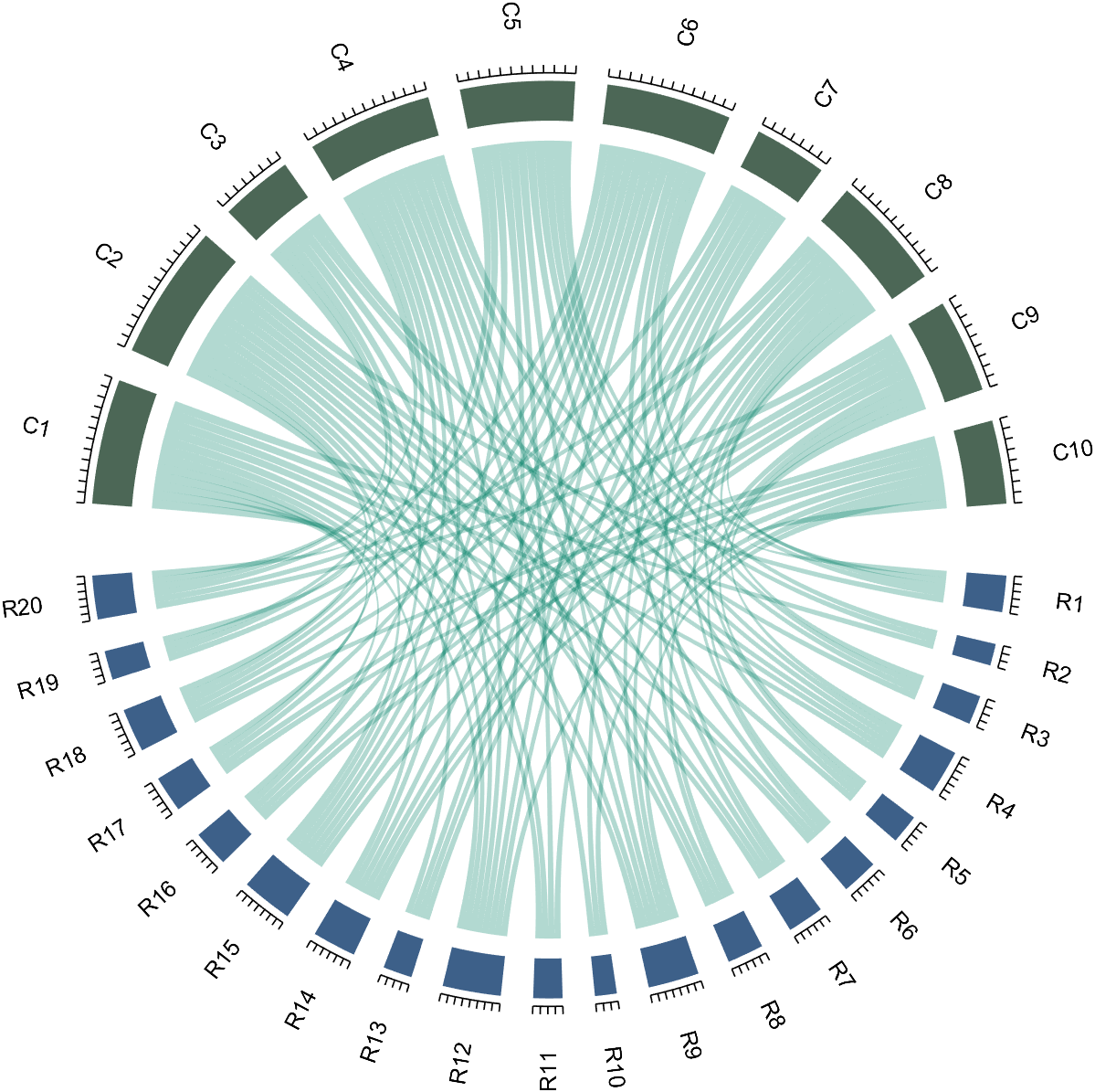
We can modify its Sep attribute:
dataMat=randi([0,1],[20,10]);
% use Sep to decrease space (separation)
% 使用 sep 减小空隙
CC=chordChart(dataMat,'Sep',1/120);
CC=CC.draw();
7 Modify Text Direction
dataMat=randi([0,1],[20,10]);
% use Sep to decrease space (separation)
% 使用 sep 减小空隙
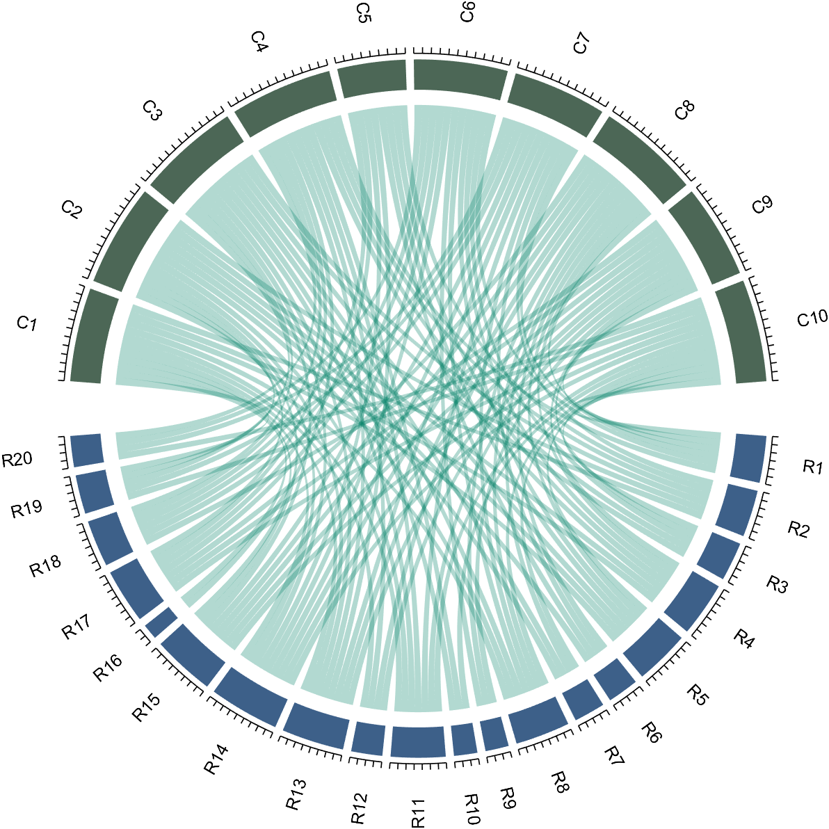
CC=chordChart(dataMat,'Sep',1/120);
CC=CC.draw();
CC.tickState('on')
% version 1.7.0更新
% 函数labelRatato用来旋转标签
% The function labelRatato is used to rotate the label
CC.labelRotate('on')
8 Add Tick Labels
dataMat=[2 0 1 2 5 1 2;
3 5 1 4 2 0 1;
4 0 5 5 2 4 3];
colName={'G1','G2','G3','G4','G5','G6','G7'};
rowName={'S1','S2','S3'};
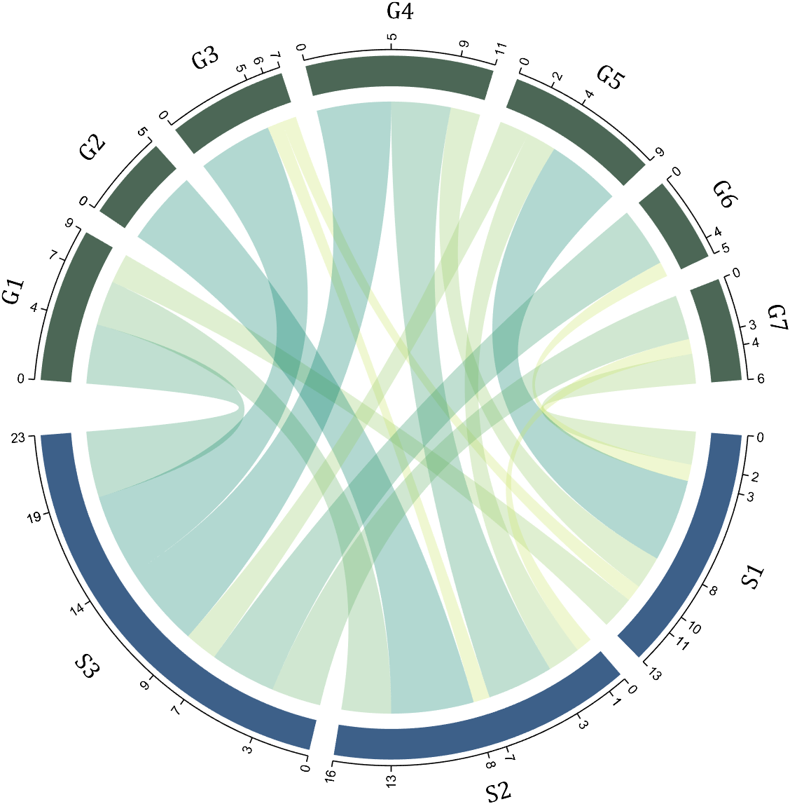
CC=chordChart(dataMat,'rowName',rowName,'colName',colName);
CC=CC.draw();
CC.setFont('FontSize',17,'FontName','Cambria')
% 显示刻度和数值
% Displays scales and numeric values
CC.tickState('on')
CC.tickLabelState('on')
% 调节标签半径
% Adjustable Label radius
CC.setLabelRadius(1.3);
% figure()
% dataMat=[2 0 1 2 5 1 2;
% 3 5 1 4 2 0 1;
% 4 0 5 5 2 4 3];
% dataMat=dataMat+rand(3,7);
% dataMat(dataMat<1)=0;
%
% CC=chordChart(dataMat,'rowName',rowName,'colName',colName);
% CC=CC.draw();
% CC.setFont('FontSize',17,'FontName','Cambria')
%
% % 显示刻度和数值
% % Displays scales and numeric values
% CC.tickState('on')
% CC.tickLabelState('on')
%
% % 调节标签半径
% % Adjustable Label radius
% CC.setLabelRadius(1.4);

9 Custom Tick Label Format
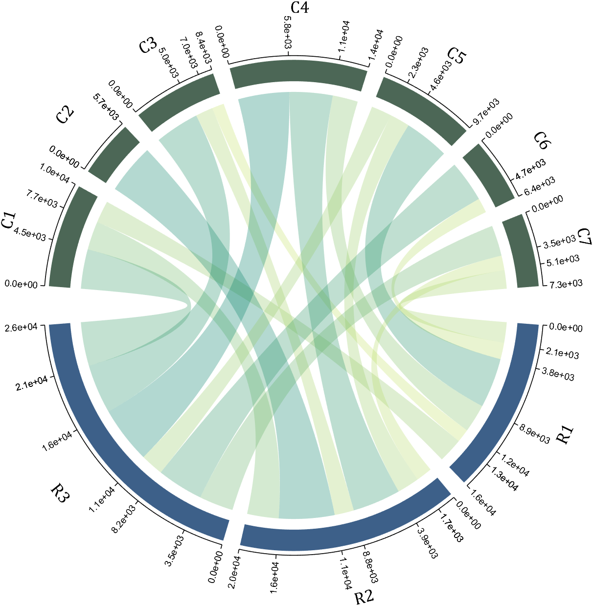
A function handle is required to input numeric output strings. The format can be set through the setTickLabelFormat function, such as Scientific notation:
dataMat=[2 0 1 2 5 1 2;
3 5 1 4 2 0 1;
4 0 5 5 2 4 3];
dataMat=dataMat+rand(3,7);
dataMat(dataMat<1)=0;
dataMat=dataMat.*1000;
CC=chordChart(dataMat);
CC=CC.draw();
CC.setFont('FontSize',17,'FontName','Cambria')
% 显示刻度和数值
% Displays scales and numeric values
CC.tickState('on')
CC.tickLabelState('on')
% 调节标签半径
% Adjustable Label radius
CC.setLabelRadius(1.4);
% 调整数值字符串格式
% Adjust numeric string format
CC.setTickLabelFormat(@(x)sprintf('%0.1e',x))
10 A Demo
rng(2)
dataMat=randi([1,7],[11,5]);
colName={'Fly','Beetle','Leaf','Soil','Waxberry'};
rowName={'Bartomella','Bradyrhizobium','Dysgomonas','Enterococcus',...
'Lactococcus','norank','others','Pseudomonas','uncultured',...
'Vibrionimonas','Wolbachia'};
CC=chordChart(dataMat,'rowName',rowName,'colName',colName,'Sep',1/80);
CC=CC.draw();
% 修改上方方块颜色(Modify the color of the blocks above)
CListT=[0.7765 0.8118 0.5216;0.4431 0.4706 0.3843;0.5804 0.2275 0.4549;
0.4471 0.4039 0.6745;0.0157 0 0 ];
for i=1:5
CC.setSquareT_N(i,'FaceColor',CListT(i,:))
end
% 修改下方方块颜色(Modify the color of the blocks below)
CListF=[0.5843 0.6863 0.7843;0.1098 0.1647 0.3255;0.0902 0.1608 0.5373;
0.6314 0.7961 0.2118;0.0392 0.2078 0.1059;0.0157 0 0 ;
0.8549 0.9294 0.8745;0.3882 0.3255 0.4078;0.5020 0.7216 0.3843;
0.0902 0.1843 0.1804;0.8196 0.2314 0.0706];
for i=1:11
CC.setSquareF_N(i,'FaceColor',CListF(i,:))
end
% 修改弦颜色(Modify chord color)
for i=1:5
for j=1:11
CC.setChordMN(j,i,'FaceColor',CListT(i,:),'FaceAlpha',.5)
end
end
CC.tickState('on')
CC.labelRotate('on')
CC.setFont('FontSize',17,'FontName','Cambria')
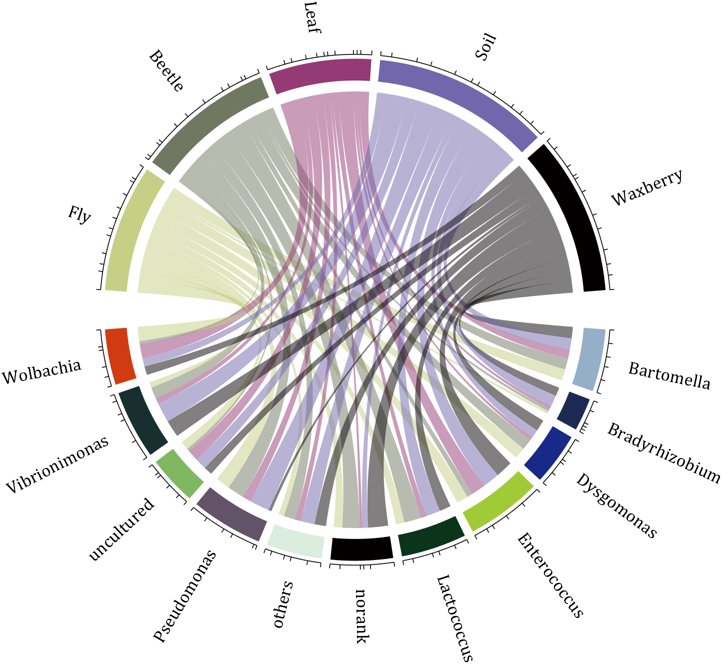
Hope to have your Reviews and Stars!!!
↓ ↓ ↓ ↓ ↓ ↓ ↓ ↓ ↓ ↓
↑ ↑ ↑ ↑ ↑ ↑ ↑ ↑ ↑ ↑
We are modeling the introduction of a novel pathogen into a completely susceptible population. In the cells below, I have provided you with the Matlab code for a simple stochastic SIR model, implemented using the "GillespieSSA" function
Simulating the stochastic model 100 times for 

Since γ is 0.4 per day,  per day
% Define the parameters
beta = 0.36;
gamma = 0.4;
n_sims = 100;
tf = 100; % Time frame changed to 100
% Calculate R0
R0 = beta / gamma
% Initial state values
initial_state_values = [1000000; 1; 0; 0]; % S, I, R, cum_inc
% Define the propensities and state change matrix
a = @(state) [beta * state(1) * state(2) / 1000000, gamma * state(2)];
nu = [-1, 0; 1, -1; 0, 1; 0, 0];
% Define the Gillespie algorithm function
function [t_values, state_values] = gillespie_ssa(initial_state, a, nu, tf)
t = 0;
state = initial_state(:); % Ensure state is a column vector
t_values = t;
state_values = state';
while t < tf
rates = a(state);
rate_sum = sum(rates);
if rate_sum == 0
break;
end
tau = -log(rand) / rate_sum;
t = t + tau;
r = rand * rate_sum;
cum_sum_rates = cumsum(rates);
reaction_index = find(cum_sum_rates >= r, 1);
state = state + nu(:, reaction_index);
% Update cumulative incidence if infection occurred
if reaction_index == 1
state(4) = state(4) + 1; % Increment cumulative incidence
end
t_values = [t_values; t];
state_values = [state_values; state'];
end
end
% Function to simulate the stochastic model multiple times and plot results
function simulate_stoch_model(beta, gamma, n_sims, tf, initial_state_values, R0, plot_type)
% Define the propensities and state change matrix
a = @(state) [beta * state(1) * state(2) / 1000000, gamma * state(2)];
nu = [-1, 0; 1, -1; 0, 1; 0, 0];
% Set random seed for reproducibility
rng(11);
% Initialize plot
figure;
hold on;
for i = 1:n_sims
[t, output] = gillespie_ssa(initial_state_values, a, nu, tf);
% Check if the simulation had only one step and re-run if necessary
while length(t) == 1
[t, output] = gillespie_ssa(initial_state_values, a, nu, tf);
end
if strcmp(plot_type, 'cumulative_incidence')
plot(t, output(:, 4), 'LineWidth', 2, 'Color', rand(1, 3));
elseif strcmp(plot_type, 'prevalence')
plot(t, output(:, 2), 'LineWidth', 2, 'Color', rand(1, 3));
end
end
xlabel('Time (days)');
if strcmp(plot_type, 'cumulative_incidence')
ylabel('Cumulative Incidence');
ylim([0 inf]);
elseif strcmp(plot_type, 'prevalence')
ylabel('Prevalence of Infection');
ylim([0 50]);
end
title(['Stochastic model output for R0 = ', num2str(R0)]);
subtitle([num2str(n_sims), ' simulations']);
xlim([0 tf]);
grid on;
hold off;
end
% Simulate the model 100 times and plot cumulative incidence
simulate_stoch_model(beta, gamma, n_sims, tf, initial_state_values, R0, 'cumulative_incidence');
% Simulate the model 100 times and plot prevalence
simulate_stoch_model(beta, gamma, n_sims, tf, initial_state_values, R0, 'prevalence');


Many times when ploting, we not only need to set the color of the plot, but also its
transparency, Then how we set the alphaData of colorbar at the same time ?
It seems easy to do so :
data = rand(12,12);
% Transparency range 0-1, .3-1 for better appearance here
AData = rescale(- data, .3, 1);
% Draw an imagesc with numerical control over colormap and transparency
imagesc(data, 'AlphaData',AData);
colormap(jet);
ax = gca;
ax.DataAspectRatio = [1,1,1];
ax.TickDir = 'out';
ax.Box = 'off';
% get colorbar object
CBarHdl = colorbar;
pause(1e-16)
% Modify the transparency of the colorbar
CData = CBarHdl.Face.Texture.CData;
ALim = [min(min(AData)), max(max(AData))];
CData(4,:) = uint8(255.*rescale(1:size(CData, 2), ALim(1), ALim(2)));
CBarHdl.Face.Texture.ColorType = 'TrueColorAlpha';
CBarHdl.Face.Texture.CData = CData;
But !!!!!!!!!!!!!!! We cannot preserve the changes when saving them as images :

It seems that when saving plots, the `Texture` will be refresh, but the `Face` will not :
however, object Face only have 4 colors to change(The four corners of a quadrilateral), how
can we set more colors ??


`Face` is a quadrilateral object, and we can change the `VertexData` to draw more than one little quadrilaterals:
data = rand(12,12);
% Transparency range 0-1, .3-1 for better appearance here
AData = rescale(- data, .3, 1);
%Draw an imagesc with numerical control over colormap and transparency
imagesc(data, 'AlphaData',AData);
colormap(jet);
ax = gca;
ax.DataAspectRatio = [1,1,1];
ax.TickDir = 'out';
ax.Box = 'off';
% get colorbar object
CBarHdl = colorbar;
pause(1e-16)
% Modify the transparency of the colorbar
CData = CBarHdl.Face.Texture.CData;
ALim = [min(min(AData)), max(max(AData))];
CData(4,:) = uint8(255.*rescale(1:size(CData, 2), ALim(1), ALim(2)));
warning off
CBarHdl.Face.ColorType = 'TrueColorAlpha';
VertexData = CBarHdl.Face.VertexData;
tY = repmat((1:size(CData,2))./size(CData,2), [4,1]);
tY1 = tY(:).'; tY2 = tY - tY(1,1); tY2(3:4,:) = 0; tY2 = tY2(:).';
tM1 = [tY1.*0 + 1; tY1; tY1.*0 + 1];
tM2 = [tY1.*0; tY2; tY1.*0];
CBarHdl.Face.VertexData = repmat(VertexData, [1,size(CData,2)]).*tM1 + tM2;
CBarHdl.Face.ColorData = reshape(repmat(CData, [4,1]), 4, []);

The higher the value, the more transparent it becomes
data = rand(12,12);
AData = rescale(- data, .3, 1);
imagesc(data, 'AlphaData',AData);
colormap(jet);
ax = gca;
ax.DataAspectRatio = [1,1,1];
ax.TickDir = 'out';
ax.Box = 'off';
CBarHdl = colorbar;
pause(1e-16)
CData = CBarHdl.Face.Texture.CData;
ALim = [min(min(AData)), max(max(AData))];
CData(4,:) = uint8(255.*rescale(size(CData, 2):-1:1, ALim(1), ALim(2)));
warning off
CBarHdl.Face.ColorType = 'TrueColorAlpha';
VertexData = CBarHdl.Face.VertexData;
tY = repmat((1:size(CData,2))./size(CData,2), [4,1]);
tY1 = tY(:).'; tY2 = tY - tY(1,1); tY2(3:4,:) = 0; tY2 = tY2(:).';
tM1 = [tY1.*0 + 1; tY1; tY1.*0 + 1];
tM2 = [tY1.*0; tY2; tY1.*0];
CBarHdl.Face.VertexData = repmat(VertexData, [1,size(CData,2)]).*tM1 + tM2;
CBarHdl.Face.ColorData = reshape(repmat(CData, [4,1]), 4, []);

More transparent in the middle
data = rand(12,12) - .5;
AData = rescale(abs(data), .1, .9);
imagesc(data, 'AlphaData',AData);
colormap(jet);
ax = gca;
ax.DataAspectRatio = [1,1,1];
ax.TickDir = 'out';
ax.Box = 'off';
CBarHdl = colorbar;
pause(1e-16)
CData = CBarHdl.Face.Texture.CData;
ALim = [min(min(AData)), max(max(AData))];
CData(4,:) = uint8(255.*rescale(abs((1:size(CData, 2)) - (1 + size(CData, 2))/2), ALim(1), ALim(2)));
warning off
CBarHdl.Face.ColorType = 'TrueColorAlpha';
VertexData = CBarHdl.Face.VertexData;
tY = repmat((1:size(CData,2))./size(CData,2), [4,1]);
tY1 = tY(:).'; tY2 = tY - tY(1,1); tY2(3:4,:) = 0; tY2 = tY2(:).';
tM1 = [tY1.*0 + 1; tY1; tY1.*0 + 1];
tM2 = [tY1.*0; tY2; tY1.*0];
CBarHdl.Face.VertexData = repmat(VertexData, [1,size(CData,2)]).*tM1 + tM2;
CBarHdl.Face.ColorData = reshape(repmat(CData, [4,1]), 4, []);

The code will work if the plot have AlphaData property
data = peaks(30);
AData = rescale(data, .2, 1);
surface(data, 'FaceAlpha','flat','AlphaData',AData);
colormap(jet(100));
ax = gca;
ax.DataAspectRatio = [1,1,1];
ax.TickDir = 'out';
ax.Box = 'off';
view(3)
CBarHdl = colorbar;
pause(1e-16)
CData = CBarHdl.Face.Texture.CData;
ALim = [min(min(AData)), max(max(AData))];
CData(4,:) = uint8(255.*rescale(1:size(CData, 2), ALim(1), ALim(2)));
warning off
CBarHdl.Face.ColorType = 'TrueColorAlpha';
VertexData = CBarHdl.Face.VertexData;
tY = repmat((1:size(CData,2))./size(CData,2), [4,1]);
tY1 = tY(:).'; tY2 = tY - tY(1,1); tY2(3:4,:) = 0; tY2 = tY2(:).';
tM1 = [tY1.*0 + 1; tY1; tY1.*0 + 1];
tM2 = [tY1.*0; tY2; tY1.*0];
CBarHdl.Face.VertexData = repmat(VertexData, [1,size(CData,2)]).*tM1 + tM2;
CBarHdl.Face.ColorData = reshape(repmat(CData, [4,1]), 4, []);

How to leave feedback on a doc page
Leaving feedback is a two-step process. At the bottom of most pages in the MATLAB documentation is a star rating.

Start by selecting a star that best answers the question. After selecting a star rating, an edit box appears where you can offer specific feedback.

When you press "Submit" you'll see the confirmation dialog below. You cannot go back and edit your content, although you can refresh the page to go through that process again.

Tips on leaving feedback
- Be productive. The reader should clearly understand what action you'd like to see, what was unclear, what you think needs work, or what areas were really helpful.
- Positive feedback is also helpful. By nature, feedback often focuses on suggestions for changes but it also helps to know what was clear and what worked well.
- Point to specific areas of the page. This helps the reader to narrow the focus of the page to the area described by your feedback.
What happens to that feedback?
Before working at MathWorks I often left feedback on documentation pages but I never knew what happens after that. One day in 2021 I shared my speculation on the process:
> That feedback is received by MathWorks Gnomes which are never seen nor heard but visit the MathWorks documentation team at night while they are sleeping and whisper selected suggestions into their ears to manipulate their dreams. Occassionally this causes them to wake up with a Eureka moment that leads to changes in the documentation.

I'd like to let you in on the secret which is much less fanciful. Feedback left in the star rating and edit box are collected and periodically reviewed by the doc writers who look for trends on highly trafficked pages and finer grain feedback on less visited pages. Your feedback is important and often results in improvements.
A colleague said that you can search the Help Center using the phrase 'Introduced in' followed by a release version. Such as, 'Introduced in R2022a'. Doing this yeilds search results specific for that release.
Seems pretty handy so I thought I'd share.
Bringing the beauty of MathWorks Natick's tulips to life through code!

Remix challenge: create and share with us your new breeds of MATLAB tulips!

This cheat sheet is here:
reference:
- https://github.com/peijin94/matlabPlotCheatsheet
- https://github.com/mathworks/visualization-cheat-sheet
- https://www.mathworks.com/products/matlab/plot-gallery.html
- https://www.mathworks.com/help/matlab/release-notes.html
MATLAB used to have official visualization-cheat-sheet, but there have been quite a few new updates in MATLAB versions recently. Therefore, I made my own cheat sheet and marked the versions of each new thing that were released :


From Alpha Vantage's website: API Documentation | Alpha Vantage
Try using the built-in Matlab function webread(URL)... for example:
% copy a URL from the examples on the site
URL = 'https://www.alphavantage.co/query?function=TIME_SERIES_DAILY&symbol=IBM&apikey=demo'
% or use the pattern to create one
tickers = [{'IBM'} {'SPY'} {'DJI'} {'QQQ'}]; i = 1;
URL = ...
['https://www.alphavantage.co/query?function=TIME_SERIES_DAILY_ADJUSTED&outputsize=full&symbol=', ...
+ tickers{i}, ...
+ '&apikey=***Put Your API Key here***'];
X = webread(URL);
You can access any of the data available on the site as per the Alpha Vantage documentation using these two lines of code but with different designations for the requested data as per the documentation.
It's fun!
How to create a legend as follows?
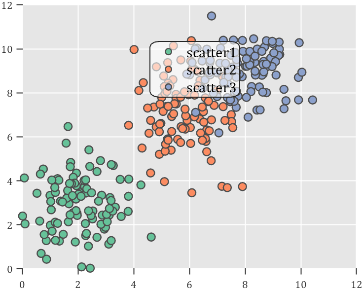

Principle Explanation - Graphic Objects
Hidden Properties of Legend are laid as follows
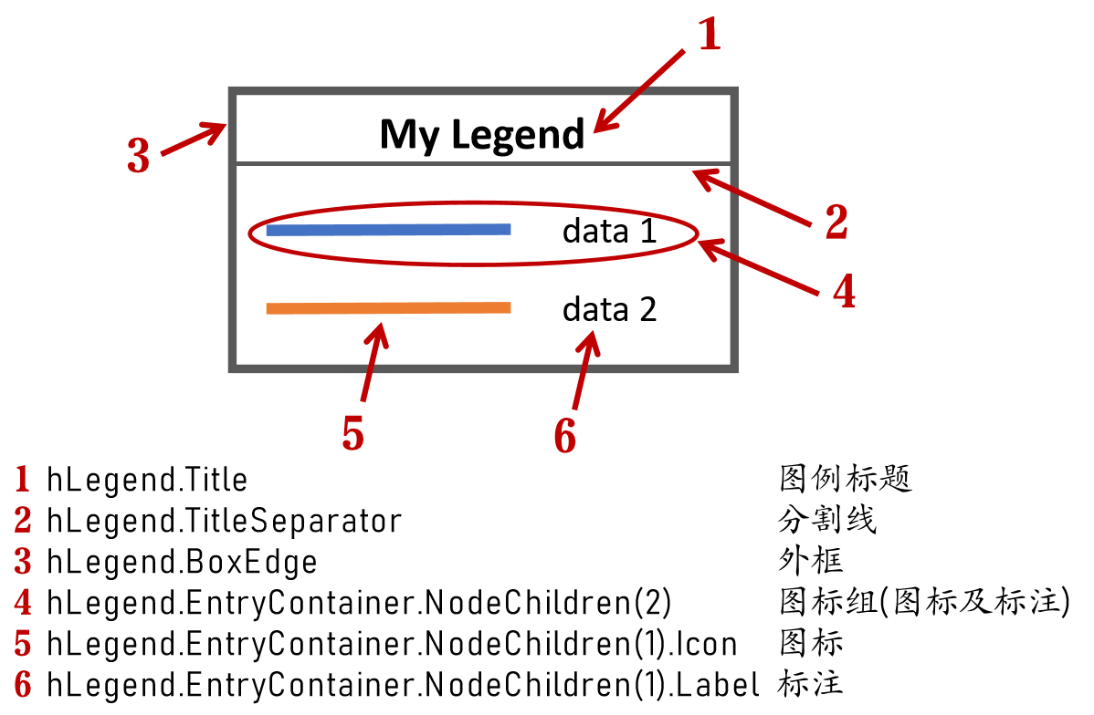
In most cases, legends are drawn using LineLoop and Quadrilateral:
Both of these basic graphic objects are drawn in groups of four points, and the general principle is as follows:

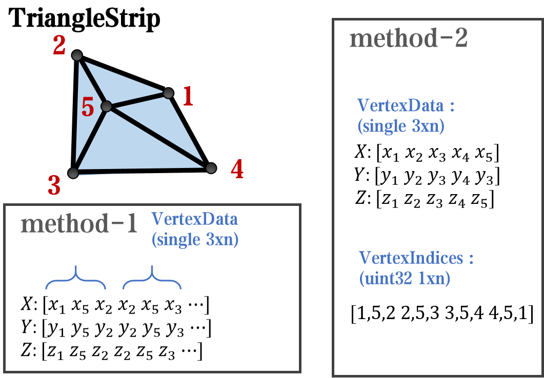
Of course, you can arrange the points in order, or set VertexIndices whitch means the vertex order to obtain the desired quadrilateral shape:

Other objects
Compared to objects that can only be grouped into four points, we also need to introduce more flexible objects. Firstly, LineStrip, a graphical object that draws lines in groups of two points:
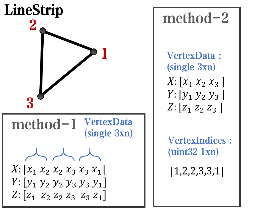
And TriangleStrip is a set of three points that draw objects to fill triangles, for example, complex polygons can be filled with multiple triangles:
Principle Explanation - Create and Replace
Let's talk about how to construct basic graphic objects, which are all constructed using undisclosed and very low-level functions, such as LineStrip, not through:
- LineStrip()
It is built through:
- matlab.graphics.primitive.world.LineStrip()
After building the object, the following properties must be set to make the hidden object visible:
- Layer
- ColorBinding
- ColorData
- VertexData
- PickableParts
The settings of these properties can refer to the original legend to form the object, which will not be elaborated here. You can also refer to the code I wrote.
Afterwards, set the newly constructed object's parent class as the Group parent class of the original component, and then hide the original component
newBoxEdgeHdl.Parent=oriBoxEdgeHdl.Parent;
oriBoxEdgeHdl.Visible='off';
The above is the entire process of component replacement, with two example codes written:
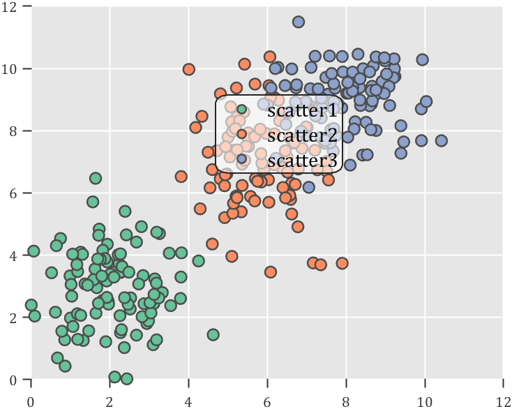
Semi transparent legend
function SPrettyLegend(lgd)
% Semitransparent rounded rectangle legend
% Copyright (c) 2023, Zhaoxu Liu / slandarer
% -------------------------------------------------------------------------
% Zhaoxu Liu / slandarer (2023). pretty legend
% (https://www.mathworks.com/matlabcentral/fileexchange/132128-pretty-legend),
% MATLAB Central File Exchange. 检索来源 2023/7/9.
% =========================================================================
if nargin<1
ax = gca;
lgd = get(ax,'Legend');
end
pause(1e-6)
Ratio = .1;
t1 = linspace(0,pi/2,4); t1 = t1([1,2,2,3,3,4]);
t2 = linspace(pi/2,pi,4); t2 = t2([1,2,2,3,3,4]);
t3 = linspace(pi,3*pi/2,4); t3 = t3([1,2,2,3,3,4]);
t4 = linspace(3*pi/2,2*pi,4); t4 = t4([1,2,2,3,3,4]);
XX = [1,1,1-Ratio+cos(t1).*Ratio,1-Ratio,Ratio,Ratio+cos(t2).*Ratio,...
0,0,Ratio+cos(t3).*Ratio,Ratio,1-Ratio,1-Ratio+cos(t4).*Ratio];
YY = [Ratio,1-Ratio,1-Ratio+sin(t1).*Ratio,1,1,1-Ratio+sin(t2).*Ratio,...
1-Ratio,Ratio,Ratio+sin(t3).*Ratio,0,0,Ratio+sin(t4).*Ratio];
% 圆角边框(border-radius)
oriBoxEdgeHdl = lgd.BoxEdge;
newBoxEdgeHdl = matlab.graphics.primitive.world.LineStrip();
newBoxEdgeHdl.AlignVertexCenters = 'off';
newBoxEdgeHdl.Layer = 'front';
newBoxEdgeHdl.ColorBinding = 'object';
newBoxEdgeHdl.LineWidth = 1;
newBoxEdgeHdl.LineJoin = 'miter';
newBoxEdgeHdl.WideLineRenderingHint = 'software';
newBoxEdgeHdl.ColorData = uint8([38;38;38;0]);
newBoxEdgeHdl.VertexData = single([XX;YY;XX.*0]);
newBoxEdgeHdl.Parent=oriBoxEdgeHdl.Parent;
oriBoxEdgeHdl.Visible='off';
% 半透明圆角背景(Semitransparent rounded background)
oriBoxFaceHdl = lgd.BoxFace;
newBoxFaceHdl = matlab.graphics.primitive.world.TriangleStrip();
Ind = [1:(length(XX)-1);ones(1,length(XX)-1).*(length(XX)+1);2:length(XX)];
Ind = Ind(:).';
newBoxFaceHdl.PickableParts = 'all';
newBoxFaceHdl.Layer = 'back';
newBoxFaceHdl.ColorBinding = 'object';
newBoxFaceHdl.ColorType = 'truecoloralpha';
newBoxFaceHdl.ColorData = uint8(255*[1;1;1;.6]);
newBoxFaceHdl.VertexData = single([XX,.5;YY,.5;XX.*0,0]);
newBoxFaceHdl.VertexIndices = uint32(Ind);
newBoxFaceHdl.Parent = oriBoxFaceHdl.Parent;
oriBoxFaceHdl.Visible = 'off';
end
Usage examples
clc; clear; close all
rng(12)
% 生成随机点(Generate random points)
mu = [2 3; 6 7; 8 9];
S = cat(3,[1 0; 0 2],[1 0; 0 2],[1 0; 0 1]);
r1 = abs(mvnrnd(mu(1,:),S(:,:,1),100));
r2 = abs(mvnrnd(mu(2,:),S(:,:,2),100));
r3 = abs(mvnrnd(mu(3,:),S(:,:,3),100));
% 绘制散点图(Draw scatter chart)
hold on
propCell = {'LineWidth',1.2,'MarkerEdgeColor',[.3,.3,.3],'SizeData',60};
scatter(r1(:,1),r1(:,2),'filled','CData',[0.40 0.76 0.60],propCell{:});
scatter(r2(:,1),r2(:,2),'filled','CData',[0.99 0.55 0.38],propCell{:});
scatter(r3(:,1),r3(:,2),'filled','CData',[0.55 0.63 0.80],propCell{:});
% 增添图例(Draw legend)
lgd = legend('scatter1','scatter2','scatter3');
lgd.Location = 'northwest';
lgd.FontSize = 14;
% 坐标区域基础修饰(Axes basic decoration)
ax=gca; grid on
ax.FontName = 'Cambria';
ax.Color = [0.9,0.9,0.9];
ax.Box = 'off';
ax.TickDir = 'out';
ax.GridColor = [1 1 1];
ax.GridAlpha = 1;
ax.LineWidth = 1;
ax.XColor = [0.2,0.2,0.2];
ax.YColor = [0.2,0.2,0.2];
ax.TickLength = [0.015 0.025];
% 隐藏轴线(Hide XY-Ruler)
pause(1e-6)
ax.XRuler.Axle.LineStyle = 'none';
ax.YRuler.Axle.LineStyle = 'none';
SPrettyLegend(lgd)
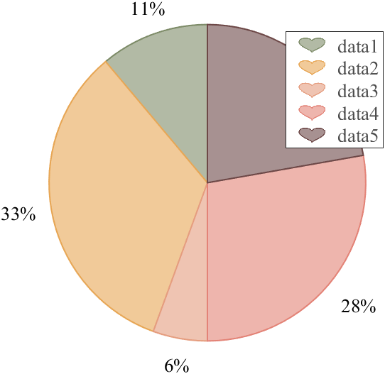
Heart shaped legend (exclusive to pie charts)
function pie2HeartLegend(lgd)
% Heart shaped legend for pie chart
% Copyright (c) 2023, Zhaoxu Liu / slandarer
% -------------------------------------------------------------------------
% Zhaoxu Liu / slandarer (2023). pretty legend
% (https://www.mathworks.com/matlabcentral/fileexchange/132128-pretty-legend),
% MATLAB Central File Exchange. 检索来源 2023/7/9.
% =========================================================================
if nargin<1
ax = gca;
lgd = get(ax,'Legend');
end
pause(1e-6)
% 心形曲线(Heart curve)
x = -1:1/100:1;
y1 = 0.6 * abs(x) .^ 0.5 + ((1 - x .^ 2) / 2) .^ 0.5;
y2 = 0.6 * abs(x) .^ 0.5 - ((1 - x .^ 2) / 2) .^ 0.5;
XX = [x, flip(x),x(1)]./3.4+.5;
YY = ([y1, y2,y1(1)]-.2)./2+.5;
Ind = [1:(length(XX)-1);2:length(XX)];
Ind = Ind(:).';
% 获取图例图标(Get Legend Icon)
lgdEntryChild = lgd.EntryContainer.NodeChildren;
iconSet = arrayfun(@(lgdEntryChild)lgdEntryChild.Icon.Transform.Children.Children,lgdEntryChild,UniformOutput=false);
% 基础边框句柄(Base Border Handle)
newEdgeHdl = matlab.graphics.primitive.world.LineStrip();
newEdgeHdl.AlignVertexCenters = 'off';
newEdgeHdl.Layer = 'front';
newEdgeHdl.ColorBinding = 'object';
newEdgeHdl.LineWidth = .8;
newEdgeHdl.LineJoin = 'miter';
newEdgeHdl.WideLineRenderingHint = 'software';
newEdgeHdl.ColorData = uint8([38;38;38;0]);
newEdgeHdl.VertexData = single([XX;YY;XX.*0]);
newEdgeHdl.VertexIndices = uint32(Ind);
% 基础多边形面句柄(Base Patch Handle)
newFaceHdl = matlab.graphics.primitive.world.TriangleStrip();
Ind = [1:(length(XX)-1);ones(1,length(XX)-1).*(length(XX)+1);2:length(XX)];
Ind = Ind(:).';
newFaceHdl.PickableParts = 'all';
newFaceHdl.Layer = 'middle';
newFaceHdl.ColorBinding = 'object';
newFaceHdl.ColorType = 'truecoloralpha';
newFaceHdl.ColorData = uint8(255*[1;1;1;.6]);
newFaceHdl.VertexData = single([XX,.5;YY,.5;XX.*0,0]);
newFaceHdl.VertexIndices = uint32(Ind);
% 替换图例图标(Replace Legend Icon)
for i = 1:length(iconSet)
oriEdgeHdl = iconSet{i}(1);
tNewEdgeHdl = copy(newEdgeHdl);
tNewEdgeHdl.ColorData = oriEdgeHdl.ColorData;
tNewEdgeHdl.Parent = oriEdgeHdl.Parent;
oriEdgeHdl.Visible = 'off';
oriFaceHdl = iconSet{i}(2);
tNewFaceHdl = copy(newFaceHdl);
tNewFaceHdl.ColorData = oriFaceHdl.ColorData;
tNewFaceHdl.Parent = oriFaceHdl.Parent;
oriFaceHdl.Visible = 'off';
end
end
Usage examples
clc; clear; close all
% 生成随机点(Generate random points)
X = [1 3 0.5 2.5 2];
pieHdl = pie(X);
% 修饰饼状图(Decorate pie chart)
colorList=[0.4941 0.5490 0.4118
0.9059 0.6510 0.3333
0.8980 0.6157 0.4980
0.8902 0.5137 0.4667
0.4275 0.2824 0.2784];
for i = 1:2:length(pieHdl)
pieHdl(i).FaceColor=colorList((i+1)/2,:);
pieHdl(i).EdgeColor=colorList((i+1)/2,:);
pieHdl(i).LineWidth=1;
pieHdl(i).FaceAlpha=.6;
end
for i = 2:2:length(pieHdl)
pieHdl(i).FontSize=13;
pieHdl(i).FontName='Times New Roman';
end
lgd=legend('FontSize',13,'FontName','Times New Roman','TextColor',[1,1,1].*.3);
pie2HeartLegend(lgd)
Temporary print statements are often helpful during debugging but it's easy to forget to remove the statements or sometimes you may not have writing privileges for the file. This tip uses conditional breakpoints to add print statements without ever editing the file!
What are conditional breakpoints?
Conditional breakpoints allow you to write a conditional statement that is executed when the selected line is hit and if the condition returns true, MATLAB pauses at that line. Otherwise, it continues.
The Hack: use ~fprintf() as the condition
fprintf prints information to the command window and returns the size of the message in bytes. The message size will always be greater than 0 which will always evaluate as true when converted to logical. Therefore, by negating an fprintf statement within a conditional breakpoint, the fprintf command will execute, print to the command window, and evalute as false which means the execution will continue uninterupted!
How to set a conditional break point
1. Right click the line number where you want the condition to be evaluated and select "Set Conditional Breakpoint"

2. Enter a valid MATLAB expression that returns a logical scalar value in the editor dialog.

Handy one-liners
Check if a line is reached: Don't forget the negation (~) and the line break (\n)!
~fprintf('Entered callback function\n')
Display the call stack from the break point line: one of my favorites!
~fprintf('%s\n',formattedDisplayText(struct2table(dbstack)))
Inspect variable values: For scalar values,
~fprintf('v = %.5f\n', v)
~fprintf('%s\n', formattedDisplayText(v)).
Make sense of frequent hits: In some situations such as responses to listeners or interactive callbacks, a line can be executed 100s of times per second. Incorporate a timestamp to differentiate messages during rapid execution.
~fprintf('WindowButtonDownFcn - %s\n', datetime('now'))
Closing
This tip not only keeps your code clean but also offers a dynamic way to monitor code execution and variable states without permanent modifications. Interested in digging deeper? @Steve Eddins takes this tip to the next level with his Code Trace for MATLAB tool available on the File Exchange (read more).
Summary animation

To reproduce the events in this animation:
% buttonDownFcnDemo.m
fig = figure();
tcl = tiledlayout(4,4,'TileSpacing','compact');
for i = 1:16
ax = nexttile(tcl);
title(ax,"#"+string(i))
ax.ButtonDownFcn = @axesButtonDownFcn;
xlim(ax,[-1 1])
ylim(ax,[-1,1])
hold(ax,'on')
end
function axesButtonDownFcn(obj,event)
colors = lines(16);
plot(obj,event.IntersectionPoint(1),event.IntersectionPoint(2),...
'ko','MarkerFaceColor',colors(obj.Layout.Tile,:))
end
If you've dabbled in "procedural generation," (algorithmically generating natural features), you may have come across the problem of sphere texturing. How to seamlessly texture a sphere is not immediately obvious. Watch what happens, for example, if you try adding power law noise to an evenly sampled grid of spherical angle coordinates (i.e. a "UV sphere" in Blender-speak):
% Example: how [not] to texture a sphere:
rng(2, 'twister'); % Make what I have here repeatable for you
% Make our radial noise, mapped onto an equal spaced longitude and latitude
% grid.
N = 51;
b = linspace(-1, 1, N).^2;
r = abs(ifft2(exp(6i*rand(N))./(b'+b+1e-5))); % Power law noise
r = rescale(r, 0, 1) + 5;
[lon, lat] = meshgrid(linspace(0, 2*pi, N), linspace(-pi/2, pi/2, N));
[x2, y2, z2] = sph2cart(lon, lat, r);
r2d = @(x)x*180/pi;
% Radial surface texture
subplot(1, 3, 1);
imagesc(r, 'Xdata', r2d(lon(1,:)), 'Ydata', r2d(lat(:, 1)));
xlabel('Longitude (Deg)');
ylabel('Latitude (Deg)');
title('Texture (radial variation)');
% View from z axis
subplot(1, 3, 2);
surf(x2, y2, z2, r);
axis equal
view([0, 90]);
title('Top view');
% Side view
subplot(1, 3, 3);
surf(x2, y2, z2, r);
axis equal
view([-90, 0]);
title('Side view');

The created surface shows "pinching" at the poles due to different radial values mapping to the same location. Furthermore, the noise statistics change based on the density of the sampling on the surface.
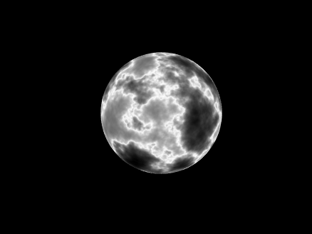
How can this be avoided? One standard method is to create a textured volume and sample the volume at points on a sphere. Code for doing this is quite simple:
rng default % Make our noise realization repeatable
% Create our 3D power-law noise
N = 201;
b = linspace(-1, 1, N);
[x3, y3, z3] = meshgrid(b, b, b);
b3 = x3.^2 + y3.^2 + z3.^2;
r = abs(ifftn(ifftshift(exp(6i*randn(size(b3)))./(b3.^1.2 + 1e-6))));
% Modify it - make it more interesting
r = rescale(r);
r = r./(abs(r - 0.5) + .1);
% Sample on a sphere
[x, y, z] = sphere(500);
% Plot
ir = interp3(x3, y3, z3, r, x, y, z, 'linear', 0);
surf(x, y, z, ir);
shading flat
axis equal off
set(gcf, 'color', 'k');
colormap(gray);
The result of evaluating this code is a seamless, textured sphere with no discontinuities at the poles or variation in the spatial statistics of the noise texture:
But what if you want to smooth it or perform some other local texture modification? Smoothing the volume and resampling is not equivalent to smoothing the surficial features shown on the map above.
A more flexible alternative is to treat the samples on the sphere surface as a set of interconnected nodes that are influenced by adjacent values. Using this approach we can start by defining the set of nodes on a sphere surface. These can be sampled almost arbitrarily, though the noise statistics will vary depending on the sampling strategy.
One noise realisation I find attractive can be had by randomly sampling a sphere. Normalizing a point in N-dimensional space by its 2-norm projects it to the surface of an N-dimensional unit sphere, so randomly sampling a sphere can be done very easily using randn() and vecnorm():
N = 5e3; % Number of nodes on our sphere
g=randn(3,N); % Random 3D points around origin
p=g./vecnorm(g); % Projected to unit sphere
The next step is to find each point's "neighbors." The first step is to find the convex hull. Since each point is on the sphere, the convex hull will include each point as a vertex in the triangulation:
k=convhull(p');
In the above, k is an N x 3 set of indices where each row represents a unique triangle formed by a triplicate of points on the sphere surface. The vertices of the full set of triangles containing a point describe the list of neighbors to that point.
What we want now is a large, sparse symmetric matrix where the indices of the columns & rows represent the indices of the points on the sphere and the nth row (and/or column) contains non-zero entries at the indices corresponding to the neighbors of the nth point.
How to do this? You could set up a tiresome nested for-loop searching for all rows (triangles) in k that contain some index n, or you could directly index via:
c=@(x)sparse(k(:,x)*[1,1,1],k,1,N,N);
t=c(1)|c(2)|c(3);
The result is the desired sparse connectivity matrix: a matrix with non-zero entries defining neighboring points.
So how do we create a textured sphere with this connectivity matrix? We will use it to form a set of equations that, when combined with the concept of "regularization," will allow us to determine the properties of the randomness on the surface. Our regularizer will penalize the difference of the radial distance of a point and the average of its neighbors. To do this we replace the main diagonal with the negative of the sum of the off-diagonal components so that the rows and columns are zero-mean. This can be done via:
w=spdiags(-sum(t,2)+1,0,double(t));
Now we invoke a bit of linear algebra. Pretend x is an N-length vector representing the radial distance of each point on our sphere with the noise realization we desire. Y will be an N-length vector of "observations" we are going to generate randomly, in this case using a uniform distribution (because it has a bias and we want a non-zero average radius, but you can play around with different distributions than uniform to get different effects):
Y=rand(N,1);
and A is going to be our "transformation" matrix mapping x to our noisy observations:
Ax = Y
In this case both x and Y are N length vectors and A is just the identity matrix:
A = speye(N);
Y, however, doesn't create the noise realization we want. So in the equation above, when solving for x we are going to introduce a regularizer which is going to penalize unwanted behavior of x by some amount. That behavior is defined by the point-neighbor radial differences represented in matrix w. Our estimate of x can then be found using one of my favorite Matlab assets, the "\" operator:
smoothness = 10; % Smoothness penalty: higher is smoother
x = (A+smoothness*w'*w)\Y; % Solving for radii
The vector x now contains the radii with the specified noise realization for the sphere which can be created simply by multiplying x by p and plotting using trisurf:
p2 = p.*x';
trisurf(k,p2(1,:),p2(2,:),p2(3,:),'FaceC', 'w', 'EdgeC', 'none','AmbientS',0,'DiffuseS',0.6,'SpecularS',1);
light;
set(gca, 'color', 'k');
axis equal
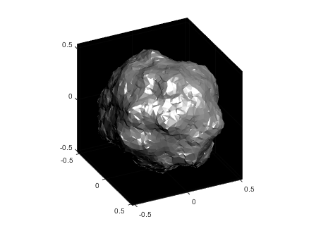
The following images show what happens as you change the smoothness parameter using values [.1, 1, 10, 100] (left to right):

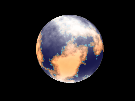
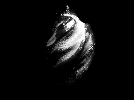
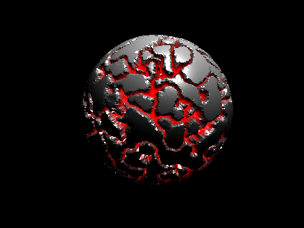
Now you know a couple ways to make a textured sphere: that's the starting point for having a lot of fun with basic procedural planet, moon, or astroid generation! Here's some examples of things you can create based on these general ideas:

I am often talking to new MATLAB users. I have put together one script. If you know how this script works, why, and what each line means, you will be well on your way on your MATLAB learning journey.
% Clear existing variables and close figures
clear;
close all;
% Print to the Command Window
disp('Hello, welcome to MATLAB!');
% Create a simple vector and matrix
vector = [1, 2, 3, 4, 5];
matrix = [1, 2, 3; 4, 5, 6; 7, 8, 9];
% Display the created vector and matrix
disp('Created vector:');
disp(vector);
disp('Created matrix:');
disp(matrix);
% Perform element-wise multiplication
result = vector .* 2;
% Display the result of the operation
disp('Result of element-wise multiplication of the vector by 2:');
disp(result);
% Create plot
x = 0:0.1:2*pi; % Generate values from 0 to 2*pi
y = sin(x); % Calculate the sine of these values
% Plotting
figure; % Create a new figure window
plot(x, y); % Plot x vs. y
title('Simple Plot of sin(x)'); % Give the plot a title
xlabel('x'); % Label the x-axis
ylabel('sin(x)'); % Label the y-axis
grid on; % Turn on the grid
disp('This is the end of the script. Explore MATLAB further to learn more!');
Introduction
Comma-separated lists are really very simple. You use them all the time. Here is one:
a,b,c,d
That is a comma-separated list containing four variables, the variables a, b, c, and d. Every time you write a list separated by commas then you are writing a comma-separated list. Most commonly you would write a comma-separated list as inputs when calling a function:
fun(a,b,c,d)
or as arguments to the concatenation operator or cell construction operator:
[a,b,c,d]
{a,b,c,d}
or as function outputs:
[a,b,c,d] = fun();
It is very important to understand that in general a comma-separated list is NOT one variable (but it could be). However, sometimes it is useful to create a comma-separated list from one variable (or define one variable from a comma-separated list), and MATLAB has several ways of doing this from various container array types:
struct_array.field % all elements
struct_array(idx).field % selected elements
cell_array{:} % all elements
cell_array{idx} % selected elements
string_array{:} % all elements
string_array{idx} % selected elements
Note that in all cases, the comma-separated list consists of the content of the container array, not subsets (or "slices") of the container array itself (use parentheses to "slice" any array). In other words, they will be equivalent to writing this comma-separated list of the container array content:
content1, content2, content3, .. , contentN
and will return as many content arrays as the original container array has elements (or that you select using indexing, in the requested order). A comma-separated list of one element is just one array, but in general there can be any number of separate arrays in the comma-separated list (zero, one, two, three, four, or more). Here is an example showing that a comma-separated list generated from the content of a cell array is the same as a comma-separated list written explicitly:
>> C = {1,0,Inf};
>> C{:}
ans =
1
ans =
0
ans =
Inf
>> 1,0,Inf
ans =
1
ans =
0
ans =
Inf
How to Use Comma-Separated Lists
Function Inputs: Remember that every time you call a function with multiple input arguments you are using a comma-separated list:
fun(a,b,c,d)
and this is exactly why they are useful: because you can specify the arguments for a function or operator without knowing anything about the arguments (even how many there are). Using the example cell array from above:
>> vertcat(C{:})
ans =
1
0
Inf
which, as we should know by now, is exactly equivalent to writing the same comma-separated list directly into the function call:
>> vertcat(1,0,Inf)
ans =
1
0
Inf
How can we use this? Commonly these are used to generate vectors of values from a structure or cell array, e.g. to concatenate the filenames which are in the output structure of dir:
S = dir(..);
F = {S.name}
which is simply equivalent to
F = {S(1).name, S(2).name, S(3).name, .. , S(end).name}
Or, consider a function with multiple optional input arguments:
opt = {'HeaderLines',2, 'Delimiter',',', 'CollectOutputs',true);
fid = fopen(..);
C = textscan(fid,'%f%f',opt{:});
fclose(fid);
Note how we can pass the optional arguments as a comma-separated list. Remember how a comma-separated list is equivalent to writing var1,var2,var3,..., then the above example is really just this:
C = textscan(fid,'%f%f', 'HeaderLines',2, 'Delimiter',',', 'CollectOutputs',true)
with the added advantage that we can specify all of the optional arguments elsewhere and handle them as one cell array (e.g. as a function input, or at the top of the file). Or we could select which options we want simply by using indexing on that cell array. Note that varargin and varargout can also be useful here.
Function Outputs: In much the same way that the input arguments can be specified, so can an arbitrary number of output arguments. This is commonly used for functions which return a variable number of output arguments, specifically ind2sub and gradient and ndgrid. For example we can easily get all outputs of ndgrid, for any number of inputs (in this example three inputs and three outputs, determined by the number of elements in the cell array):
C = {1:3,4:7,8:9};
[C{:}] = ndgrid(C{:});
which is thus equivalent to:
[C{1},C{2},C{3}] = ndgrid(C{1},C{2},C{3});
Further Topics:
MATLAB documentation:
Click on these links to jump to relevant comments below:
Dynamic Indexing (indexing into arrays with arbitrary numbers of dimensions)
Summary
Just remember that in general a comma-separated list is not one variable (although they can be), and that they are exactly what they say: a list (of arrays) separated with commas. You use them all the time without even realizing it, every time you write this:
fun(a,b,c,d)


The beautiful and elegant chord diagrams were all created using MATLAB?
Indeed, they were all generated using the chord diagram plotting toolkit that I developed myself:
- - Chord chart: [chord chart](https://www.mathworks.com/matlabcentral/fileexchange/116550-chord-chart)
- - Directed graph chord chart: [digraph chord chart]:(https://www.mathworks.com/matlabcentral/fileexchange/121043-digraph-chord-chart)
You can download these toolkits from the provided links.
The reason for writing this article is that many people have started using the chord diagram plotting toolkit that I developed. However, some users are unsure about customizing certain styles. As the developer, I have a good understanding of the implementation principles of the toolkit and can apply it flexibly. This has sparked the idea of challenging myself to create various styles of chord diagrams. Currently, the existing code is quite lengthy. In the future, I may integrate some of this code into the toolkit, enabling users to achieve the effects of many lines of code with just a few lines.
Without further ado, let's see the extent to which this MATLAB toolkit can currently perform.
demo 1


rng(2)
dataMat = randi([0,5], [11,5]);
dataMat(1:6,1) = 0;
dataMat([11,7],1) = [45,25];
dataMat([1,4,5,7],2) = [20,20,30,30];
dataMat(:,3) = 0;
dataMat(6,3) = 45;
dataMat(1:5,4) = 0;
dataMat([6,7],4) = [25,25];
dataMat([5,6,9],5) = [25,25,25];
colName = {'Fly', 'Beetle', 'Leaf', 'Soil', 'Waxberry'};
rowName = {'Bartomella', 'Bradyrhizobium', 'Dysgomonas', 'Enterococcus',...
'Lactococcus', 'norank', 'others', 'Pseudomonas', 'uncultured',...
'Vibrionimonas', 'Wolbachia'};
figure('Units','normalized', 'Position',[.02,.05,.6,.85])
CC = chordChart(dataMat, 'rowName',rowName, 'colName',colName, 'Sep',1/80);
CC = CC.draw();
% 修改上方方块颜色(Modify the color of the blocks above)
CListT = [0.7765 0.8118 0.5216; 0.4431 0.4706 0.3843; 0.5804 0.2275 0.4549;
0.4471 0.4039 0.6745; 0.0157 0 0 ];
for i = 1:size(dataMat, 2)
CC.setSquareT_N(i, 'FaceColor',CListT(i,:))
end
% 修改下方方块颜色(Modify the color of the blocks below)
CListF = [0.5843 0.6863 0.7843; 0.1098 0.1647 0.3255; 0.0902 0.1608 0.5373;
0.6314 0.7961 0.2118; 0.0392 0.2078 0.1059; 0.0157 0 0 ;
0.8549 0.9294 0.8745; 0.3882 0.3255 0.4078; 0.5020 0.7216 0.3843;
0.0902 0.1843 0.1804; 0.8196 0.2314 0.0706];
for i = 1:size(dataMat, 1)
CC.setSquareF_N(i, 'FaceColor',CListF(i,:))
end
% 修改弦颜色(Modify chord color)
for i = 1:size(dataMat, 1)
for j = 1:size(dataMat, 2)
CC.setChordMN(i,j, 'FaceColor',CListT(j,:), 'FaceAlpha',.5)
end
end
CC.tickState('on')
CC.labelRotate('on')
CC.setFont('FontSize',17, 'FontName','Cambria')
% CC.labelRotate('off')
% textHdl = findobj(gca,'Tag','ChordLabel');
% for i = 1:length(textHdl)
% if textHdl(i).Position(2) < 0
% if abs(textHdl(i).Position(1)) > .7
% textHdl(i).Rotation = textHdl(i).Rotation + 45;
% textHdl(i).HorizontalAlignment = 'right';
% if textHdl(i).Rotation > 90
% textHdl(i).Rotation = textHdl(i).Rotation + 180;
% textHdl(i).HorizontalAlignment = 'left';
% end
% else
% textHdl(i).Rotation = textHdl(i).Rotation + 10;
% textHdl(i).HorizontalAlignment = 'right';
% end
% end
% end
demo 2

rng(3)
dataMat = randi([1,15], [7,22]);
dataMat(dataMat < 11) = 0;
dataMat(1, sum(dataMat, 1) == 0) = 15;
colName = {'A2M', 'FGA', 'FGB', 'FGG', 'F11', 'KLKB1', 'SERPINE1', 'VWF',...
'THBD', 'TFPI', 'PLAT', 'SERPINA5', 'SERPIND1', 'F2', 'PLG', 'F12',...
'SERPINC1', 'SERPINA1', 'PROS1', 'SERPINF2', 'F13A1', 'PROC'};
rowName = {'Lung', 'Spleen', 'Liver', 'Heart',...
'Renal cortex', 'Renal medulla', 'Thyroid'};
figure('Units','normalized', 'Position',[.02,.05,.6,.85])
CC = chordChart(dataMat, 'rowName',rowName, 'colName',colName, 'Sep',1/80, 'LRadius',1.21);
CC = CC.draw();
CC.labelRotate('on')
% 单独设置每一个弦末端方块(Set individual end blocks for each chord)
% Use obj.setEachSquareF_Prop
% or obj.setEachSquareT_Prop
% F means from (blocks below)
% T means to (blocks above)
CListT = [173,70,65; 79,135,136]./255;
% Upregulated:1 | Downregulated:2
Regulated = rand([7, 22]);
Regulated = (Regulated < .8) + 1;
for i = 1:size(Regulated, 1)
for j = 1:size(Regulated, 2)
CC.setEachSquareT_Prop(i, j, 'FaceColor', CListT(Regulated(i,j),:))
end
end
% 绘制图例(Draw legend)
H1 = fill([0,1,0] + 100, [1,0,1] + 100, CListT(1,:), 'EdgeColor','none');
H2 = fill([0,1,0] + 100, [1,0,1] + 100, CListT(2,:), 'EdgeColor','none');
lgdHdl = legend([H1,H2], {'Upregulated','Downregulated'}, 'AutoUpdate','off', 'Location','best');
lgdHdl.ItemTokenSize = [12,12];
lgdHdl.Box = 'off';
lgdHdl.FontSize = 13;
% 修改下方方块颜色(Modify the color of the blocks below)
CListF = [128,108,171; 222,208,161; 180,196,229; 209,150,146; 175,201,166;
134,156,118; 175,175,173]./255;
for i = 1:size(dataMat, 1)
CC.setSquareF_N(i, 'FaceColor',CListF(i,:))
end
% 修改弦颜色(Modify chord color)
for i = 1:size(dataMat, 1)
for j = 1:size(dataMat, 2)
CC.setChordMN(i,j, 'FaceColor',CListF(i,:), 'FaceAlpha',.45)
end
end
demo 3

dataMat = rand([15,15]);
dataMat(dataMat > .15) = 0;
CList = [ 75,146,241; 252,180, 65; 224, 64, 10; 5,100,146; 191,191,191;
26, 59,105; 255,227,130; 18,156,221; 202,107, 75; 0, 92,219;
243,210,136; 80, 99,129; 241,185,168; 224,131, 10; 120,147,190]./255;
figure('Units','normalized', 'Position',[.02,.05,.6,.85])
BCC = biChordChart(dataMat, 'Arrow','on', 'CData',CList);
BCC = BCC.draw();
% 添加刻度
BCC.tickState('on')
% 修改字体,字号及颜色
BCC.setFont('FontName','Cambria', 'FontSize',17, 'Color',[0,0,.8])
demo 4


rng(5)
dataMat = randi([1,20], [5,5]);
dataMat(1,1) = 110;
dataMat(2,2) = 40;
dataMat(3,3) = 50;
dataMat(5,5) = 50;
CList1 = [164,190,158; 216,213,153; 177,192,208; 238,238,227; 249,217,153]./255;
CList2 = [247,204,138; 128,187,185; 245,135,124; 140,199,197; 252,223,164]./255;
CList = CList2;
NameList={'CHORD','CHART','MADE','BY','SLANDARER'};
figure('Units','normalized', 'Position',[.02,.05,.6,.85])
BCC = biChordChart(dataMat, 'Arrow','on', 'CData',CList, 'Sep',1/30, 'Label',NameList, 'LRadius',1.33);
BCC = BCC.draw();
% 添加刻度
BCC.tickState('on')
% 修改弦颜色(Modify chord color)
for i = 1:size(dataMat, 1)
for j = 1:size(dataMat, 2)
if dataMat(i,j) > 0
BCC.setChordMN(i,j, 'FaceAlpha',.7, 'EdgeColor',CList(i,:)./1.1)
end
end
end
% 修改方块颜色(Modify the color of the blocks)
for i = 1:size(dataMat, 1)
BCC.setSquareN(i, 'EdgeColor',CList(i,:)./1.7)
end
% 修改字体,字号及颜色
BCC.setFont('FontName','Cambria', 'FontSize',17)
BCC.tickLabelState('on')
BCC.setTickFont('FontName','Cambria', 'FontSize',9)
demo 5

dataMat=randi([1,20], [14,3]);
dataMat(11:14,1) = 0;
dataMat(6:10,2) = 0;
dataMat(1:5,3) = 0;
colName = compose('C%d', 1:3);
rowName = [compose('A%d', 1:7), compose('B%d', 7:-1:1)];
figure('Units','normalized', 'Position',[.02,.05,.6,.85])
CC = chordChart(dataMat, 'rowName',rowName, 'colName',colName, 'Sep',1/80);
CC = CC.draw();
% 修改上方方块颜色(Modify the color of the blocks above)
for i = 1:size(dataMat, 2)
CC.setSquareT_N(i, 'FaceColor',[190,190,190]./255)
end
% 修改下方方块颜色(Modify the color of the blocks below)
CListF=[255,244,138; 253,220,117; 254,179, 78; 253,190, 61;
252, 78, 41; 228, 26, 26; 178, 0, 36; 4, 84,119;
1,113,137; 21,150,155; 67,176,173; 68,173,158;
123,204,163; 184,229,162]./255;
for i = 1:size(dataMat, 1)
CC.setSquareF_N(i, 'FaceColor',CListF(i,:))
end
% 修改弦颜色(Modify chord color)
for i = 1:size(dataMat, 1)
for j = 1:size(dataMat, 2)
CC.setChordMN(i,j, 'FaceColor',CListF(i,:), 'FaceAlpha',.5)
end
end
CC.tickState('on')
CC.tickLabelState('on')
demo 6

rng(2)
dataMat = randi([0,40], [20,4]);
dataMat(rand([20,4]) < .2) = 0;
dataMat(1,3) = 500;
dataMat(20,1:4) = [140; 150; 80; 90];
colName = compose('T%d', 1:4);
rowName = compose('SL%d', 1:20);
figure('Units','normalized', 'Position',[.02,.05,.6,.85])
CC = chordChart(dataMat, 'rowName',rowName, 'colName',colName, 'Sep',1/80, 'LRadius',1.23);
CC = CC.draw();
% 修改上方方块颜色(Modify the color of the blocks above)
CListT = [0.62,0.49,0.27; 0.28,0.57,0.76
0.25,0.53,0.30; 0.86,0.48,0.34];
for i = 1:size(dataMat, 2)
CC.setSquareT_N(i, 'FaceColor',CListT(i,:))
end
% 修改下方方块颜色(Modify the color of the blocks below)
CListF = [0.94,0.84,0.60; 0.16,0.50,0.67; 0.92,0.62,0.49;
0.48,0.44,0.60; 0.48,0.44,0.60; 0.71,0.79,0.73;
0.96,0.98,0.98; 0.51,0.82,0.95; 0.98,0.70,0.82;
0.97,0.85,0.84; 0.55,0.64,0.62; 0.94,0.93,0.60;
0.98,0.90,0.85; 0.72,0.84,0.81; 0.85,0.45,0.49;
0.76,0.76,0.84; 0.59,0.64,0.62; 0.62,0.14,0.15;
0.75,0.75,0.75; 1.00,1.00,1.00];
for i = 1:size(dataMat, 1)
CC.setSquareF_N(i, 'FaceColor',CListF(i,:))
end
CC.setSquareF_N(size(dataMat, 1), 'EdgeColor','k', 'LineWidth',1)
% 修改弦颜色(Modify chord color)
for i = 1:size(dataMat, 1)
for j = 1:size(dataMat, 2)
CC.setChordMN(i,j, 'FaceColor',CListT(j,:), 'FaceAlpha',.46)
end
end
CC.tickState('on')
CC.labelRotate('on')
CC.setFont('FontSize',17, 'FontName','Cambria')
demo 7

dataMat = randi([10,10000], [10,10]);
dataMat(6:10,:) = 0;
dataMat(:,1:5) = 0;
NameList = {'BOC', 'ICBC', 'ABC', 'BOCM', 'CCB', ...
'yama', 'nikoto', 'saki', 'koto', 'kawa'};
CList = [0.63,0.75,0.88
0.67,0.84,0.75
0.85,0.78,0.88
1.00,0.92,0.93
0.92,0.63,0.64
0.57,0.67,0.75
1.00,0.65,0.44
0.72,0.73,0.40
0.65,0.57,0.58
0.92,0.94,0.96];
figure('Units','normalized', 'Position',[.02,.05,.6,.85])
BCC = biChordChart(dataMat, 'Arrow','on', 'CData',CList, 'Label',NameList);
BCC = BCC.draw();
% 修改弦颜色(Modify chord color)
for i = 1:size(dataMat, 1)
for j = 1:size(dataMat, 2)
if dataMat(i,j) > 0
BCC.setChordMN(i,j, 'FaceAlpha',.85, 'EdgeColor',CList(i,:)./1.5, 'LineWidth',.8)
end
end
end
for i = 1:size(dataMat, 1)
BCC.setSquareN(i, 'EdgeColor',CList(i,:)./1.5, 'LineWidth',1)
end
% 添加刻度、修改字体
BCC.tickState('on')
BCC.setFont('FontName','Cambria', 'FontSize',17)
demo 8

dataMat = rand([11,4]);
dataMat = round(10.*dataMat.*((11:-1:1).'+1))./10;
colName = {'A','B','C','D'};
rowName = {'Acidobacteriota', 'Actinobacteriota', 'Proteobacteria', ...
'Chloroflexi', 'Bacteroidota', 'Firmicutes', 'Gemmatimonadota', ...
'Verrucomicrobiota', 'Patescibacteria', 'Planctomyetota', 'Others'};
figure('Units','normalized', 'Position',[.02,.05,.8,.85])
CC = chordChart(dataMat, 'colName',colName, 'Sep',1/80, 'SSqRatio',30/100);% -30/100
CC = CC.draw();
% 修改上方方块颜色(Modify the color of the blocks above)
CListT = [0.93,0.60,0.62
0.55,0.80,0.99
0.95,0.82,0.18
1.00,0.81,0.91];
for i = 1:size(dataMat, 2)
CC.setSquareT_N(i, 'FaceColor',CListT(i,:))
end
% 修改下方方块颜色(Modify the color of the blocks below)
CListF = [0.75,0.73,0.86
0.56,0.83,0.78
0.00,0.60,0.20
1.00,0.49,0.02
0.78,0.77,0.95
0.59,0.24,0.36
0.98,0.51,0.45
0.96,0.55,0.75
0.47,0.71,0.84
0.65,0.35,0.16
0.40,0.00,0.64];
for i = 1:size(dataMat, 1)
CC.setSquareF_N(i, 'FaceColor',CListF(i,:))
end
% 修改弦颜色(Modify chord color)
CListC = [0.55,0.83,0.76
0.75,0.73,0.86
0.00,0.60,0.19
1.00,0.51,0.04];
for i = 1:size(dataMat, 1)
for j = 1:size(dataMat, 2)
CC.setChordMN(i,j, 'FaceColor',CListC(j,:), 'FaceAlpha',.4)
end
end
% 单独设置每一个弦末端方块(Set individual end blocks for each chord)
% Use obj.setEachSquareF_Prop
% or obj.setEachSquareT_Prop
% F means from (blocks below)
% T means to (blocks above)
for i = 1:size(dataMat, 1)
for j = 1:size(dataMat, 2)
CC.setEachSquareT_Prop(i,j, 'FaceColor', CListF(i,:))
end
end
% 添加刻度
CC.tickState('on')
% 修改字体,字号及颜色
CC.setFont('FontName','Cambria', 'FontSize',17)
% 隐藏下方标签
textHdl = findobj(gca, 'Tag','ChordLabel');
for i = 1:length(textHdl)
if textHdl(i).Position(2) < 0
set(textHdl(i), 'Visible','off')
end
end
% 绘制图例(Draw legend)
scatterHdl = scatter(10.*ones(size(dataMat,1)),10.*ones(size(dataMat,1)), ...
55, 'filled');
for i = 1:length(scatterHdl)
scatterHdl(i).CData = CListF(i,:);
end
lgdHdl = legend(scatterHdl, rowName, 'Location','best', 'FontSize',16, 'FontName','Cambria', 'Box','off');
set(lgdHdl, 'Position',[.7482,.3577,.1658,.3254])
demo 9


dataMat = randi([0,10], [5,5]);
CList1 = [0.70,0.59,0.67
0.62,0.70,0.62
0.81,0.75,0.62
0.80,0.62,0.56
0.62,0.65,0.65];
CList2 = [0.02,0.02,0.02
0.59,0.26,0.33
0.38,0.49,0.38
0.03,0.05,0.03
0.29,0.28,0.32];
CList = CList2;
NameList={'CHORD','CHART','MADE','BY','SLANDARER'};
figure('Units','normalized', 'Position',[.02,.05,.6,.85])
BCC = biChordChart(dataMat, 'Arrow','on', 'CData',CList, 'Sep',1/30, 'Label',NameList, 'LRadius',1.33);
BCC = BCC.draw();
% 修改弦颜色(Modify chord color)
for i = 1:size(dataMat, 1)
for j = 1:size(dataMat, 2)
BCC.setChordMN(i,j, 'FaceAlpha',.5)
end
end
% 修改方块颜色(Modify the color of the blocks)
for i = 1:size(dataMat, 1)
BCC.setSquareN(i, 'EdgeColor',[0,0,0], 'LineWidth',5)
end
% 添加刻度
BCC.tickState('on')
% 修改字体,字号及颜色
BCC.setFont('FontSize',17, 'FontWeight','bold')
BCC.tickLabelState('on')
BCC.setTickFont('FontSize',9)
demo 10


rng(2)
dataMat = rand([14,5]) > .3;
colName = {'phosphorylation', 'vasculature development', 'blood vessel development', ...
'cell adhesion', 'plasma membrane'};
rowName = {'THY1', 'FGF2', 'MAP2K1', 'CDH2', 'HBEGF', 'CXCR4', 'ECSCR',...
'ACVRL1', 'RECK', 'PNPLA6', 'CDH5', 'AMOT', 'EFNB2', 'CAV1'};
figure('Units','normalized', 'Position',[.02,.05,.9,.85])
CC = chordChart(dataMat, 'colName',colName, 'rowName',rowName, 'Sep',1/80, 'LRadius',1.2);
CC = CC.draw();
% 修改上方方块颜色(Modify the color of the blocks above)
CListT1 = [0.5686 0.1961 0.2275
0.2275 0.2863 0.3765
0.8431 0.7882 0.4118
0.4275 0.4510 0.2706
0.3333 0.2706 0.2510];
CListT2 = [0.4941 0.5490 0.4118
0.9059 0.6510 0.3333
0.8980 0.6157 0.4980
0.8902 0.5137 0.4667
0.4275 0.2824 0.2784];
CListT3 = [0.4745 0.5843 0.7569
0.4824 0.5490 0.5843
0.6549 0.7216 0.6510
0.9412 0.9216 0.9059
0.9804 0.7608 0.6863];
CListT = CListT3;
for i = 1:size(dataMat, 2)
CC.setSquareT_N(i, 'FaceColor',CListT(i,:), 'EdgeColor',[0,0,0])
end
% 修改弦颜色(Modify chord color)
for i = 1:size(dataMat, 1)
for j = 1:size(dataMat, 2)
CC.setChordMN(i,j, 'FaceColor',CListT(j,:), 'FaceAlpha',.9, 'EdgeColor',[0,0,0])
end
end
% 修改下方方块颜色(Modify the color of the blocks below)
logFC = sort(rand(1,14))*6 - 3;
for i = 1:size(dataMat, 1)
CC.setSquareF_N(i, 'CData',logFC(i), 'FaceColor','flat', 'EdgeColor',[0,0,0])
end
CMap = [ 0 0 1.0000; 0.0645 0.0645 1.0000; 0.1290 0.1290 1.0000; 0.1935 0.1935 1.0000
0.2581 0.2581 1.0000; 0.3226 0.3226 1.0000; 0.3871 0.3871 1.0000; 0.4516 0.4516 1.0000
0.5161 0.5161 1.0000; 0.5806 0.5806 1.0000; 0.6452 0.6452 1.0000; 0.7097 0.7097 1.0000
0.7742 0.7742 1.0000; 0.8387 0.8387 1.0000; 0.9032 0.9032 1.0000; 0.9677 0.9677 1.0000
1.0000 0.9677 0.9677; 1.0000 0.9032 0.9032; 1.0000 0.8387 0.8387; 1.0000 0.7742 0.7742
1.0000 0.7097 0.7097; 1.0000 0.6452 0.6452; 1.0000 0.5806 0.5806; 1.0000 0.5161 0.5161
1.0000 0.4516 0.4516; 1.0000 0.3871 0.3871; 1.0000 0.3226 0.3226; 1.0000 0.2581 0.2581
1.0000 0.1935 0.1935; 1.0000 0.1290 0.1290; 1.0000 0.0645 0.0645; 1.0000 0 0];
colormap(CMap);
try clim([-3,3]),catch,end
try caxis([-3,3]),catch,end
CBHdl = colorbar();
CBHdl.Position = [0.74,0.25,0.02,0.2];
% =========================================================================
% 交换XY轴(Swap XY axis)
patchHdl = findobj(gca, 'Type','patch');
for i = 1:length(patchHdl)
tX = patchHdl(i).XData;
tY = patchHdl(i).YData;
patchHdl(i).XData = tY;
patchHdl(i).YData = - tX;
end
txtHdl = findobj(gca, 'Type','text');
for i = 1:length(txtHdl)
txtHdl(i).Position([1,2]) = [1,-1].*txtHdl(i).Position([2,1]);
if txtHdl(i).Position(1) < 0
txtHdl(i).HorizontalAlignment = 'right';
else
txtHdl(i).HorizontalAlignment = 'left';
end
end
lineHdl = findobj(gca, 'Type','line');
for i = 1:length(lineHdl)
tX = lineHdl(i).XData;
tY = lineHdl(i).YData;
lineHdl(i).XData = tY;
lineHdl(i).YData = - tX;
end
% =========================================================================
txtHdl = findobj(gca, 'Type','text');
for i = 1:length(txtHdl)
if txtHdl(i).Position(1) > 0
txtHdl(i).Visible = 'off';
end
end
text(1.25,-.15, 'LogFC', 'FontSize',16)
text(1.25,1, 'Terms', 'FontSize',16)
patchHdl = [];
for i = 1:size(dataMat, 2)
patchHdl(i) = fill([10,11,12],[10,13,13], CListT(i,:), 'EdgeColor',[0,0,0]);
end
lgdHdl = legend(patchHdl, colName, 'Location','best', 'FontSize',14, 'FontName','Cambria', 'Box','off');
lgdHdl.Position = [.735,.53,.167,.27];
lgdHdl.ItemTokenSize = [18,8];
demo 11

rng(2)
dataMat = rand([12,12]);
dataMat(dataMat < .85) = 0;
dataMat(7,:) = 1.*(rand(1,12)+.1);
dataMat(11,:) = .6.*(rand(1,12)+.1);
dataMat(12,:) = [2.*(rand(1,10)+.1), 0, 0];
CList = [repmat([49,49,49],[10,1]); 235,28,34; 19,146,241]./255;
figure('Units','normalized', 'Position',[.02,.05,.6,.85])
BCC = biChordChart(dataMat, 'Arrow','off', 'CData',CList);
BCC = BCC.draw();
% 添加刻度
BCC.tickState('on')
% 修改字体,字号及颜色
BCC.setFont('FontName','Cambria', 'FontSize',17)
% 修改弦颜色(Modify chord color)
for i = 1:size(dataMat, 1)
for j = 1:size(dataMat, 2)
if dataMat(i,j) > 0
BCC.setChordMN(i,j, 'FaceAlpha',.78, 'EdgeColor',[0,0,0])
end
end
end
% 修改方块颜色(Modify the color of the blocks)
for i = 1:size(dataMat, 1)
BCC.setSquareN(i, 'EdgeColor',[0,0,0], 'LineWidth',2)
end
demo 12

dataMat = rand([9,9]);
dataMat(dataMat > .7) = 0;
dataMat(eye(9) == 1) = (rand([1,9])+.2).*3;
CList = [0.85,0.23,0.24
0.96,0.39,0.18
0.98,0.63,0.22
0.99,0.80,0.26
0.70,0.76,0.21
0.24,0.74,0.71
0.27,0.65,0.84
0.09,0.37,0.80
0.64,0.40,0.84];
figure('Units','normalized', 'Position',[.02,.05,.6,.85])
BCC = biChordChart(dataMat, 'Arrow','on', 'CData',CList);
BCC = BCC.draw();
% 添加刻度、刻度标签
BCC.tickState('on')
% 修改字体,字号及颜色
BCC.setFont('FontName','Cambria', 'FontSize',17)
% 修改弦颜色(Modify chord color)
for i = 1:size(dataMat, 1)
for j = 1:size(dataMat, 2)
if dataMat(i,j) > 0
BCC.setChordMN(i,j, 'FaceAlpha',.7)
end
end
end
demo 13

rng(2)
dataMat = randi([1,40], [7,4]);
dataMat(rand([7,4]) < .1) = 0;
colName = compose('MATLAB%d', 1:4);
rowName = compose('SL%d', 1:7);
figure('Units','normalized', 'Position',[.02,.05,.7,.85])
CC = chordChart(dataMat, 'rowName',rowName, 'colName',colName, 'Sep',1/80, 'LRadius',1.32);
CC = CC.draw();
% 修改上方方块颜色(Modify the color of the blocks above)
CListT = [0.49,0.64,0.53
0.75,0.39,0.35
0.80,0.74,0.42
0.40,0.55,0.66];
for i = 1:size(dataMat, 2)
CC.setSquareT_N(i, 'FaceColor',CListT(i,:))
end
% 修改下方方块颜色(Modify the color of the blocks below)
CListF = [0.91,0.91,0.97
0.62,0.95,0.66
0.91,0.61,0.20
0.54,0.45,0.82
0.99,0.76,0.81
0.91,0.85,0.83
0.53,0.42,0.43];
for i = 1:size(dataMat, 1)
CC.setSquareF_N(i, 'FaceColor',CListF(i,:))
end
% 修改弦颜色(Modify chord color)
for i = 1:size(dataMat, 1)
for j = 1:size(dataMat, 2)
CC.setChordMN(i,j, 'FaceColor',CListT(j,:), 'FaceAlpha',.46)
end
end
CC.tickState('on')
CC.tickLabelState('on')
CC.setFont('FontSize',17, 'FontName','Cambria')
CC.setTickFont('FontSize',8, 'FontName','Cambria')
% 绘制图例(Draw legend)
scatterHdl = scatter(10.*ones(size(dataMat,1)),10.*ones(size(dataMat,1)), ...
55, 'filled');
for i = 1:length(scatterHdl)
scatterHdl(i).CData = CListF(i,:);
end
lgdHdl = legend(scatterHdl, rowName, 'Location','best', 'FontSize',16, 'FontName','Cambria', 'Box','off');
set(lgdHdl, 'Position',[.77,.38,.1658,.27])
demo 14

rng(6)
dataMat = randi([1,20], [8,8]);
dataMat(dataMat > 5) = 0;
dataMat(1,:) = randi([1,15], [1,8]);
dataMat(1,8) = 40;
dataMat(8,8) = 60;
dataMat = dataMat./sum(sum(dataMat));
CList = [0.33,0.53,0.86
0.94,0.50,0.42
0.92,0.58,0.30
0.59,0.47,0.45
0.37,0.76,0.82
0.82,0.68,0.29
0.75,0.62,0.87
0.43,0.69,0.57];
NameList={'CHORD', 'CHART', 'AND', 'BICHORD',...
'CHART', 'MADE', 'BY', 'SLANDARER'};
figure('Units','normalized', 'Position',[.02,.05,.6,.85])
BCC = biChordChart(dataMat, 'Arrow','on', 'CData',CList, 'Sep',1/12, 'Label',NameList, 'LRadius',1.33);
BCC = BCC.draw();
% 添加刻度
BCC.tickState('on')
% 修改弦颜色(Modify chord color)
for i = 1:size(dataMat, 1)
for j = 1:size(dataMat, 2)
if dataMat(i,j) > 0
BCC.setChordMN(i,j, 'FaceAlpha',.7, 'EdgeColor',CList(i,:)./1.1)
end
end
end
% 修改方块颜色(Modify the color of the blocks)
for i = 1:size(dataMat, 1)
BCC.setSquareN(i, 'EdgeColor',CList(i,:)./1.7)
end
% 修改字体,字号及颜色
BCC.setFont('FontName','Cambria', 'FontSize',17)
BCC.tickLabelState('on')
BCC.setTickFont('FontName','Cambria', 'FontSize',9)
% 调整数值字符串格式
% Adjust numeric string format
BCC.setTickLabelFormat(@(x)[num2str(round(x*100)),'%'])
demo 15

CList = [0.81,0.72,0.83
0.69,0.82,0.89
0.17,0.44,0.64
0.70,0.85,0.55
0.03,0.57,0.13
0.97,0.67,0.64
0.84,0.09,0.12
1.00,0.80,0.46
0.98,0.52,0.01
];
figure('Units','normalized', 'Position',[.02,.05,.53,.85], 'Color',[1,1,1])
% =========================================================================
ax1 = axes('Parent',gcf, 'Position',[0,1/2,1/2,1/2]);
dataMat = rand([9,9]);
dataMat(dataMat > .4) = 0;
BCC = biChordChart(dataMat, 'Arrow','on', 'CData',CList);
BCC = BCC.draw();
BCC.tickState('on')
BCC.setFont('Visible','off')
% 修改弦颜色(Modify chord color)
for i = 1:size(dataMat, 1)
for j = 1:size(dataMat, 2)
if dataMat(i,j) > 0
BCC.setChordMN(i,j, 'FaceAlpha',.6)
end
end
end
text(-1.2,1.2, 'a', 'FontName','Times New Roman', 'FontSize',35)
% =========================================================================
ax2 = axes('Parent',gcf, 'Position',[1/2,1/2,1/2,1/2]);
dataMat = rand([9,9]);
dataMat(dataMat > .4) = 0;
dataMat = dataMat.*(1:9);
BCC = biChordChart(dataMat, 'Arrow','on', 'CData',CList);
BCC = BCC.draw();
BCC.tickState('on')
BCC.setFont('Visible','off')
% 修改弦颜色(Modify chord color)
for i = 1:size(dataMat, 1)
for j = 1:size(dataMat, 2)
if dataMat(i,j) > 0
BCC.setChordMN(i,j, 'FaceAlpha',.6)
end
end
end
text(-1.2,1.2, 'b', 'FontName','Times New Roman', 'FontSize',35)
% =========================================================================
ax3 = axes('Parent',gcf, 'Position',[0,0,1/2,1/2]);
dataMat = rand([9,9]);
dataMat(dataMat > .4) = 0;
dataMat = dataMat.*(1:9).';
BCC = biChordChart(dataMat, 'Arrow','on', 'CData',CList);
BCC = BCC.draw();
BCC.tickState('on')
BCC.setFont('Visible','off')
% 修改弦颜色(Modify chord color)
for i = 1:size(dataMat, 1)
for j = 1:size(dataMat, 2)
if dataMat(i,j) > 0
BCC.setChordMN(i,j, 'FaceAlpha',.6)
end
end
end
text(-1.2,1.2, 'c', 'FontName','Times New Roman', 'FontSize',35)
% =========================================================================
ax4 = axes('Parent',gcf, 'Position',[1/2,0,1/2,1/2]);
ax4.XColor = 'none'; ax4.YColor = 'none';
ax4.XLim = [-1,1]; ax4.YLim = [-1,1];
hold on
NameList = {'Food supply', 'Biodiversity', 'Water quality regulation', ...
'Air quality regulation', 'Erosion control', 'Carbon storage', ...
'Water retention', 'Recreation', 'Soil quality regulation'};
patchHdl = [];
for i = 1:size(dataMat, 2)
patchHdl(i) = fill([10,11,12],[10,13,13], CList(i,:), 'EdgeColor',[0,0,0]);
end
lgdHdl = legend(patchHdl, NameList, 'Location','best', 'FontSize',14, 'FontName','Cambria', 'Box','off');
lgdHdl.Position = [.625,.11,.255,.27];
lgdHdl.ItemTokenSize = [18,8];
demo 16


dataMat = rand([15,15]);
dataMat(dataMat > .2) = 0;
CList = [ 75,146,241; 252,180, 65; 224, 64, 10; 5,100,146; 191,191,191;
26, 59,105; 255,227,130; 18,156,221; 202,107, 75; 0, 92,219;
243,210,136; 80, 99,129; 241,185,168; 224,131, 10; 120,147,190]./255;
CListC = [54,69,92]./255;
CList = CList.*.6 + CListC.*.4;
figure('Units','normalized', 'Position',[.02,.05,.6,.85])
BCC = biChordChart(dataMat, 'Arrow','on', 'CData',CList);
BCC = BCC.draw();
% 添加刻度
BCC.tickState('on')
% 修改字体,字号及颜色
BCC.setFont('FontName','Cambria', 'FontSize',17, 'Color',[0,0,0])
% 修改弦颜色(Modify chord color)
for i = 1:size(dataMat, 1)
for j = 1:size(dataMat, 2)
if dataMat(i,j) > 0
BCC.setChordMN(i,j, 'FaceColor',CListC ,'FaceAlpha',.07)
end
end
end
[~, N] = max(sum(dataMat > 0, 2));
for j = 1:size(dataMat, 2)
BCC.setChordMN(N,j, 'FaceColor',CList(N,:) ,'FaceAlpha',.6)
end
You need to download following tools:
- - Chord chart: [chord chart](https://www.mathworks.com/matlabcentral/fileexchange/116550-chord-chart)
- - Directed graph chord chart: [digraph chord chart]:(https://www.mathworks.com/matlabcentral/fileexchange/121043-digraph-chord-chart)
Summary:
Dynamically accessing variable names can negatively impact the readability of your code and can cause it to run slower by preventing MATLAB from optimizing it as well as it could if you used alternate techniques. The most common alternative is to use simple and efficient indexing.
Explanation:
Sometimes beginners (and some self-taught professors) think it would be a good idea to dynamically create or access variable names, the variables are often named something like these:
- matrix1, matrix2, matrix3, matrix4, ...
- test_20kmh, test_50kmh, test_80kmh, ...
- nameA, nameB, nameC, nameD,...
Good reasons why dynamic variable names should be avoided:
- Slow
- Buggy
- Security Risk
- Difficult to Work With
- Obfuscated Code Intent
- Confuses Data with Code
- Code Helper Tools do not Work
- Magically Making Variables Appear in a Workspace is Risky
There are much better alternatives to accessing dynamic variable names:
- Indexing into Cell Array or ND-Array
- Non-scalar Structures (with Indexing)
- Dynamic Field-Names in a Structure
- load into a Structure, not into the Workspace
- save the Fields of a Scalar Structure
- Use a table or timetable Array
- Use more Efficient Ways to Pass Variables Between Workspaces
Note that avoiding eval (and assignin, etc.) is not some esoteric MATLAB restriction, it also applies to many other programming languages as well:
MATLAB Documentation:
If you are not interested in reading the answers below then at least read MATLAB's own documentation on this topic Alternatives to the eval Function, which states "A frequent use of the eval function is to create sets of variables such as A1, A2, ..., An, but this approach does not use the array processing power of MATLAB and is not recommended. The preferred method is to store related data in a single array." Data in a single array can be accessed very efficiently using indexing.
Note that all of these problems and disadvantages also apply to functions load (without an output variable), assignin, evalin, and evalc, and the MATLAB documentation explicitly recommends to "Avoid functions such as eval, evalc, evalin, and feval(fname)".
The official MATLAB blogs explain why eval should be avoided, the better alternatives to eval, and clearly recommend against magically creating variables. Using eval comes out at position number one on this list of Top 10 MATLAB Code Practices That Make Me Cry. Experienced MATLAB users recommend avoiding using eval for trivial code, and have written extensively on this topic.
The line integral  , where C is the boundary of the square
  oriented counterclockwise, can be evaluated in two ways:
 , where C is the boundary of the square
 Using the definition of the line integral:
% Initialize the integral sum
integral_sum = 0;
% Segment C1: x = -1, y goes from -1 to 1
y = linspace(-1, 1);
x = -1 * ones(size(y));
dy = diff(y);
integral_sum = integral_sum + sum(-x(1:end-1) .* dy);
% Segment C2: y = 1, x goes from -1 to 1
x = linspace(-1, 1);
y = ones(size(x));
dx = diff(x);
integral_sum = integral_sum + sum(y(1:end-1).^2 .* dx);
% Segment C3: x = 1, y goes from 1 to -1
y = linspace(1, -1);
x = ones(size(y));
dy = diff(y);
integral_sum = integral_sum + sum(-x(1:end-1) .* dy);
% Segment C4: y = -1, x goes from 1 to -1
x = linspace(1, -1);
y = -1 * ones(size(x));
dx = diff(x);
integral_sum = integral_sum + sum(y(1:end-1).^2 .* dx);
disp(['Direct Method Integral: ', num2str(integral_sum)]);
Plotting the square path
% Define the square's vertices
vertices = [-1 -1; -1 1; 1 1; 1 -1; -1 -1];
% Plot the square
figure;
plot(vertices(:,1), vertices(:,2), '-o');
title('Square Path for Line Integral');
xlabel('x');
ylabel('y');
grid on;
axis equal;
% Add arrows to indicate the path direction (counterclockwise)
hold on;
for i = 1:size(vertices,1)-1
% Calculate direction
dx = vertices(i+1,1) - vertices(i,1);
dy = vertices(i+1,2) - vertices(i,2);
% Reduce the length of the arrow for better visibility
scale = 0.2;
dx = scale * dx;
dy = scale * dy;
% Calculate the start point of the arrow
startx = vertices(i,1) + (1 - scale) * dx;
starty = vertices(i,2) + (1 - scale) * dy;
% Plot the arrow
quiver(startx, starty, dx, dy, 'MaxHeadSize', 0.5, 'Color', 'r', 'AutoScale', 'off');
end
hold off;

Apply Green's Theorem for the line integral
% Define the partial derivatives of P and Q
f = @(x, y) -1 - 2*y; % derivative of -x with respect to x is -1, and derivative of y^2 with respect to y is 2y
% Compute the double integral over the square [-1,1]x[-1,1]
integral_value = integral2(f, -1, 1, 1, -1);
disp(['Green''s Theorem Integral: ', num2str(integral_value)]);
Plotting the vector field related to Green’s theorem
% Define the grid for the vector field
[x, y] = meshgrid(linspace(-2, 2, 20), linspace(-2 ,2, 20));
% Define the vector field components
P = y.^2; % y^2 component
Q = -x; % -x component
% Plot the vector field
figure;
quiver(x, y, P, Q, 'b');
hold on; % Hold on to plot the square on the same figure
% Define the square's vertices
vertices = [-1 -1; -1 1; 1 1; 1 -1; -1 -1];
% Plot the square path
plot(vertices(:,1), vertices(:,2), '-o', 'Color', 'k'); % 'k' for black color
title('Vector Field (P = y^2, Q = -x) with Square Path');
xlabel('x');
ylabel('y');
axis equal;
% Add arrows to indicate the path direction (counterclockwise)
for i = 1:size(vertices,1)-1
% Calculate direction
dx = vertices(i+1,1) - vertices(i,1);
dy = vertices(i+1,2) - vertices(i,2);
% Reduce the length of the arrow for better visibility
scale = 0.2;
dx = scale * dx;
dy = scale * dy;
% Calculate the start point of the arrow
startx = vertices(i,1) + (1 - scale) * dx;
starty = vertices(i,2) + (1 - scale) * dy;
% Plot the arrow
quiver(startx, starty, dx, dy, 'MaxHeadSize', 0.5, 'Color', 'r', 'AutoScale', 'off');
end
hold off;

To solve a surface integral for example the over the sphere
  easily in MATLAB, you can leverage the symbolic toolbox for a direct and clear solution. Here is a tip to simplify the process:
 over the sphere
 - Use Symbolic Variables and Functions: Define your variables symbolically, including the parameters of your spherical coordinates θ and ϕ and the radius r . This allows MATLAB to handle the expressions symbolically, making it easier to manipulate and integrate them.
- Express in Spherical Coordinates Directly: Since you already know the sphere's equation and the relationship in spherical coordinates, define x, y, and z in terms of r , θ and ϕ directly.
- Perform Symbolic Integration: Use MATLAB's `int` function to integrate symbolically. Since the sphere and the function
 are symmetric, you can exploit these symmetries to simplify the calculation.
Here’s how you can apply this tip in MATLAB code:
% Include the symbolic math toolbox
syms theta phi
% Define the limits for theta and phi
theta_limits = [0, pi];
phi_limits = [0, 2*pi];
% Define the integrand function symbolically
integrand = 16 * sin(theta)^3 * cos(phi)^2;
% Perform the symbolic integral for the surface integral
surface_integral = int(int(integrand, theta, theta_limits(1), theta_limits(2)), phi, phi_limits(1), phi_limits(2));
% Display the result of the surface integral symbolically
disp(['The surface integral of x^2 over the sphere is ', char(surface_integral)]);
% Number of points for plotting
num_points = 100;
% Define theta and phi for the sphere's surface
[theta_mesh, phi_mesh] = meshgrid(linspace(double(theta_limits(1)), double(theta_limits(2)), num_points), ...
linspace(double(phi_limits(1)), double(phi_limits(2)), num_points));
% Spherical to Cartesian conversion for plotting
r = 2; % radius of the sphere
x = r * sin(theta_mesh) .* cos(phi_mesh);
y = r * sin(theta_mesh) .* sin(phi_mesh);
z = r * cos(theta_mesh);
% Plot the sphere
figure;
surf(x, y, z, 'FaceColor', 'interp', 'EdgeColor', 'none');
colormap('jet'); % Color scheme
shading interp; % Smooth shading
camlight headlight; % Add headlight-type lighting
lighting gouraud; % Use Gouraud shading for smooth color transitions
title('Sphere: x^2 + y^2 + z^2 = 4');
xlabel('x-axis');
ylabel('y-axis');
zlabel('z-axis');
colorbar; % Add color bar to indicate height values
axis square; % Maintain aspect ratio to be square
view([-30, 20]); % Set a nice viewing angle

Most of my projects are the tension between what exists and what I must create to make the project work. The more I leverage what exists, the faster I can complete my project in a shorter amount of time. I often find out later in the process that a MATLAB function already exists and has existed for 10 releases. The faster that I discover built-in functions, the faster I can get to the new stuff that I have to invent.
I asked the AI Chat Playground why to use MATLAB's builtin functions and I got some interesting ideas. What are your thoughts?
AI Chat Playground:
- Efficiency and Performance: MATLAB's built-in functions are highly optimized for performance. They are written in optimized and compiled languages like C or C++, which means they run faster than equivalent functions written directly in MATLAB language. When you use these functions, your code can execute more efficiently, which is especially beneficial for handling large datasets or complex mathematical computations.
- Reliability and Stability: Built-in functions have been rigorously tested and debugged by the developers at MathWorks (the company behind MATLAB). They are less likely to contain errors compared to custom-written code, which means you can rely on them to produce accurate and consistent results.
- Ease of Use: Built-in functions are designed to be user-friendly, with clear documentation and support materials available. This can make it easier to perform complex operations without needing a deep understanding of the underlying algorithms. It also reduces the amount of code you need to write and debug, saving time and reducing the potential for errors.
- Compatibility: Built-in functions are updated alongside MATLAB itself, ensuring compatibility with new features and versions of the software. Using built-in functions can help ensure that your code continues to work correctly as MATLAB evolves.
- Advanced Features: MATLAB’s built-in functions often include advanced features and options that are not readily available or would be difficult to implement on your own. For example, MATLAB’s mathematical functions can handle a wide range of special cases and data types, providing more flexibility than custom implementations.
- Community and Support: Using built-in functions means you're working with standard tools recognized by the MATLAB community. This can make it easier to get help from other users or from MathWorks support, as more people will be familiar with the functionality and potential issues of these functions.
The community is very helpful, yet I feel really powerless that I cannot find the appropriate way to code, nor find the problems with the codes I have written. I have read numerous books on MATLAB, mostly related with science and engineering applications. Any advice to improve would be greatly appreciated. Thanks.


