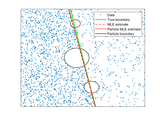
Interface detection in point cloud data (SRM & SMLM)
SMLM_interface_detection
Code for detecting interfaces in super-resolution microscopy (SRM) data, typically single-molecule localization microscopy (SMLM).
The code provided here is under Copyright © 2021 Dingeman van der Haven and Pim van der Hoorn
This method is explained in detail in the publication "Parameterless detection of liquid-liquid interfaces with sub-micron resolution in single-molecule localization microscopy", 2022, https://doi.org/10.1016/j.jcis.2022.03.116
Brief explanation for using the scripts for determining the MLE for the boundary between two regions of a Poisson Point Process with different densities in each region.
The model assumption is that the points come from a Poisson Point Process on a rectangular region. This region has been divided into two regions by a straight line through the point [a] and [b] and the Poisson process is homogeneous in both regions but with different density values. See figure below:
				a
			------------------------
			|	\		|
			|	 \		|
			|	  \	   mu2	|
			|	   \		|
			|  mu1	    \		|
			|	     \		|
			|	      \		|
			------------------------
					b
To generate an instance of the Poisson Point Process use [generatePoisson2D]. Here you need to specify the points [a] and [b] for the line that separates the two regions. You also need to specify the expected number of points [M] and the relative density [delta] between mu1 and mu2.
The main function is [mleBoundaryEstimation]. This computes the maximum value of the loglikelihood estimator and outputs the estimated separation line that maximizes the loglikelihood as well as the maximum value of the likelihood function.
To compute the MLE the function only considers lines through pairs of points(p1, p2) that lie in a given top bandwith and bottom bandwidth:
		top bandwidth
			------------------------
			|     |			|
			|     |			|
			|_____|			|
			|	   		|
			|  	 _______	|
			|	|	|	|
			|	|    	|	|
			------------------------
			  bottom bandwidth
Both the boundaries of the top bandwidth and the bottom bandwidth can be specified using the optional second and third argument of [mleBoundaryEstimation].
There are two main computation modes available that determine which points in the specified boundaries are considered. These can be set via the [IterationMethod] parameter:
Steps:
For this the parameter [IterationMethod] should be set to 'steps'. This is also the default setting for [mleBoundaryEstimation]. In this mode the boundaries of both the top and bottom bandwidth that intersect with the boundaries of the region, are partitioned into equal size intervals. This means, for example, that if the provided bandwidth overlaps with the left and top boundary of the region the left boundary of the bandwidth and the top boundary will be partitioned.
The number of intervals can be specified using the [IterationSteps] parameter. If [IterationSteps] is set to M, then there will be M+1 points (the +1 is for one of the boundaries). The default setting is 50.
The MLE estimation will then consider lines that go through the pair of points (p1, p2), where p1 is one of the interval boundaries for the partitioned top bandwidth and p2 an interval boundary in the bottom bandwidth
			   p1
			|-|-|-|-----------------
			T     |			|
		 p1 	T     |			|
			T_____|			|
			|	   		|
			|   	    _____	|
			|   	   |	 |	|
			|   	   |	 |	|
			-----------|-|-|-|------
				   p2
Points:
For this the parameter [IterationMethod] should be set to 'points'. With this setting the MLE is computed by considering lines that go through pairs of points (p1, p2), where p1 and p2 are points of the Poisson process in the top and bottom bandwidth, respectively.
			------------------------
			|     |			|
			|  p1 |			|
			|_____|			|
			|			|
			|  	 _______	|
			|	|	|	|
			|	|   p2 	|	|
			------------------------
The script [testBoundaryEstimation] provides a minimal code example for running the estimation procedure.
Note: The script mleBoundaryEstimationParticle currently does not account for overlap between the particles at the interface. If the particles at the interface overlap, the overlap area between two particles will be subtracted from the left and/or right area twice, which should not happen. This needs to be corrected in a future version by checking all particle pairs for overlap and then making sure that the overlap between the particles is only subtracted once.
Citation pour cette source
Danny van der Haven (2026). Interface detection in point cloud data (SRM & SMLM) (https://github.com/DLHvdH/SMLM_interface_detection/releases/tag/v1.0), GitHub. Extrait(e) le .
Compatibilité avec les versions de MATLAB
Plateformes compatibles
Windows macOS LinuxTags
Découvrir Live Editor
Créez des scripts avec du code, des résultats et du texte formaté dans un même document exécutable.
| Version | Publié le | Notes de version | |
|---|---|---|---|
| 1.0 |


