Design and Simulating Autonomy for Construction Vehicles - MATLAB
Video Player is loading.
Current Time 0:00
Duration 0:00
Loaded: 0%
Stream Type LIVE
Remaining Time 0:00
 
1x
  • Chapters
  • descriptions off, selected
  • captions off, selected
      Video length is 50:56

      Design and Simulating Autonomy for Construction Vehicles

      Overview

      Similar to commercial carmakers, makers of construction, mining, heavy-duty and off-road vehicles are actively adding autonomy or AI co-pilots to their vehicles. Engineers working on those off-road applications often need to address challenges specific to off-road operating conditions that are very different from those in self-driving cars. Those challenges include the impact of off-road motion on perception sensors, and the necessity of combining forward and backward motions to go to certain restricted places. In this webinar, we will use an autonomous construction vehicle as an example to show how to use MATLAB and Simulink to develop and customize autonomy for off-road vehicles. We will show testing and optimization of the autonomous algorithms through a co-simulation between Simulink and popular game engines. 

      Highlights

      In this webinar, we will use an autonomous construction vehicle simulation example to show how to

      • Create a map of the environment and determine the location of the vehicle even given noisy sensor readings
      • Use algorithms to plan a vehicle’s path given the vehicle’s dynamic constraints and operator’s preferences
      • Develop real-time motion control for obstacle avoidance and safe operation
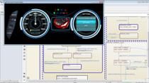
      • Establish co-simulation between Simulink and virtual environments built in game engines, such as Unity, using ROS for communication
      • Customize the algorithms to address common constraints in different off-road scenarios

      About the Presenters

      Michelle Valente joined MathWorks in 2021 as an application engineer. She specializes in Computer vision, AI and Autonomous Systems. Prior to joining MathWorks, she worked as a research engineer developing perception algorithms for robotics applications. She holds a Ph.D. in Robotics from MINES Paristech.

      Christoph Kammer is an application engineer at MathWorks in Switzerland. He supports customers in the robotics and autonomous systems domain in the areas of control and optimization, virtual scenario simulation and digital twin as well as machine and deep learning. Christoph has a master’s degree in Mechanical Engineering from ETH Zürich and a Ph.D. in Electrical Engineering from EPFL, where he specialized in control design and the control and modelling of electromechanical systems and power systems.

      Julia Antoniou is a senior application engineer for the aerospace and defense industry at MathWorks. She specializes in modeling and simulation of physical systems, with a focus on robotic and autonomous systems. Prior to joining MathWorks in 2017, Julia worked at companies such as iRobot and Johnson & Johnson in their mechanical engineering, systems engineering, and manufacturing engineering departments. Julia holds B.S. and M.S. degrees in mechanical engineering from Northeastern University.

      You Wu is a robotics evangelist and the Principal Robotics Industry Manager at MathWorks, promoting best practices in robot development processes to industrial customers. Dr. Wu received his M.S. and Ph.D. degrees in robotics from MIT and a Bachelor’s degree from Purdue University. Before joining MathWorks in 2020, he was CTO of Watchtower Robotics, a startup that deployed inspection robots into municipal water pipe networks.

      Recorded: 15 Mar 2023

      Hello, everyone. Welcome to the MathWorks webinar on Design and Simulating Autonomy for Construction Vehicles. My name is You Wu. I'm the Principal Robotics Industry Manager at MathWorks. I lead customer conversations on the best practices in robotics development process.

      I received my PhD degree in robotics from MIT. Today, I'll be the facilitator. I have my colleague Michele, Julia, and Christoph here to share their experience on adding autonomy to a construction vehicle. Let's introduce ourself first.

      Hi, everyone. My name is Michele Valente and I'm an application engineer for robotics and autonomous systems in MathWorks France. I have been at MathWorks for almost three years now. I have a PhD on mapping and localization for autonomous vehicles, and my job at MathWorks is to help customers on how MATLAB and Simulink can be used on their robotics projects. Today, I'll be covering the cost simulation infrastructure and the mapping aspect of autonomy for construction vehicles.

      Hello, everyone. My name is Julia Antoniou. I'm a senior application engineer at MathWorks, and I've been at MathWorks for five years. My job is all about working closely with engineers like you all, helping you evaluate if and how MATLAB and Simulink can help you accomplish your project goals.

      And over the past couple of years, one of my technical focus areas has been in path planning for autonomous vehicles, but specifically vehicles that operate off typical roads, like construction vehicles. So I've been working on putting together examples of how MathWorks tools can help you all that are working in this space.

      My name is Christoph Kammer. I'm an application engineer at MathWorks in Switzerland. I studied mechanical engineering at ETH Zurich, and during my PhD, I focused a lot on controls. And now at MathWorks, I focus on robotics and autonomous systems, and I recently also started to delve more into virtual environments, like Unity, and of course, all the cool new simulation workflows they enable.

      Thank you, Michelle, Julia, and Christoph. Let's talk about construction vehicles. What are the challenges in adding autonomy to those vehicles? In our observation, there are at least three. First of all, those are heavy, big vehicles. How do we create a test environment for them so that we can capture the variations in the operation condition and test safely?

      Second, how do we do motion planning for those big vehicles in this complex environment? It needs to be safe, and the same time, understand what the operator wants it to do. Third, how do we do motion planning for those vehicles? We have to satisfied all the vehicle dynamic constraints, such as turning radius, going forward, going backward. Michelle, how are we going to address those challenges?

      To address this challenge, we developed an application using MATLAB and Simulink that controls a vehicle in a construction environment. Using this app, we can define where we want the vehicle to go, we can create its trajectory, and visualize its location and sensor data, but how does this app work?

      We developed four main functionalities on it. The first one is to connect to a video environment to perform simulation. We can also visualize a map of the environment and the localization of the vehicle. Then we can plan the path to move from one point to another. And finally, we can launch the path following that we will control the vehicle. Let me show you now where this functionality is located inside the app.

      The first one is connection to the user environment. Well, for this, all we need to do is to click on Initialize ROS connection. This will establish a connection with the same ROS network as a simulator. It will also initialize the necessary subscribers and publishers for the communication between the app and the simulator.

      The next functionality is mapping and localization. Inside the app, we can load a new map of the construction site by clicking on Load New Map. The map is a bird's eye view of the construction site environment. And to make the visualization easier, we overlaid the original image with the obstacles that were detected in the map. We can see them in red. However, it's important to know that below this interface, we have a map that is in the format that can be interpreted by a robot.

      We can also localize the vehicle in the app. For this, we take the information of the vehicle position that is sent by the simulator using ROS. When we click on Enable Path Planning, we can observe that the position of the vehicle will be plotted in the map. In this application, we have the perfect position of the vehicle given by the simulator, but we could also get information of localization from other sensors like GPS.

      The next functionality is path planning. Well, now that we have clicked on Enable Path Planning, all we need to do is to select the path plan that we want and click on the position in the map where we want the vehicle to move to. Once the position is defined, we can click on Plan Path. This will call the path planner that's going to generate the path, and we're able to see it on the map.

      The last step is to control the vehicle to follow the path. For this, we only need to click on Start Path Following, which will send the plan trajectory to the controller that is in the simulator and it will control the vehicle. On the right, we have the view from the simulator, and on the app, we can also observe the vehicle moving on its trajectory.

      Now that we have seen how the app works, we're going to go through each of these functionalities and we'll show you how this was developed using MATLAB and Simulink. Let's start by the connection to the virtual environment. Do you know that we can perform code simulation between MATLAB, Simulink, and other simulators? The idea is that we can take the advantage of graph rendering and the physics of simulators to test the models and algorithms that we develop in MATLAB and Simulink.

      There are different options when it comes to simulators that we can connect to. The first one is to use the simulator that is already developed by MathWorks. It's called Simulink 3D Animation, and we can use it to create and visualize the simulation of dynamic systems.

      The second option is to use the external game engine Unreal, which is a powerful tool for creating a realistic virtual environment. Inside MATLAB and Simulink, we can find a direct interface to communicate that directly with Unreal, which makes very easy this co-simulation between Simulink, MATLAB, and Unreal environment.

      The third option is to connect to external simulators where the communication can be done by ROS, as for example, Unity and Gazebo. For this application, we use the last option. We created our scene in the Unity environment and we communicated through ROS with MATLAB and Simulink.

      Let's see now how the construction site environment was created in Unity. We imported 3D models of different vehicles such as wheel loaders, forklifts, backhoes, and trucks. We also asking different scene assets that you can find in a typical construction site. For example, buildings under construction, containers, and rocks. And to make it more realistic, we also modeled the ground of this type of environment.

      As our goal is to make a construction machine autonomous, we also needed to add sensors for the machine to perceive the environment. So what type of sensors we added to the machine? Well, as a first perception sensor, we added a camera to the front of the vehicle. The camera in this type of application can be very useful to detect information in the scene as, for example, other vehicles, people working in the construction site, or even potholes that a vehicle needs to avoid.

      We also added a LIDAR to the top of the vehicle so it can have a 360-degree view of the environment. This sensor can be used to detect the distance to other obstacles and to create a precise map of the construction site. Finally, we also add an IMU to help to estimate the localization of the vehicle.

      So now that we have all the elements in Unity, let's see how we can make our machine autonomous using MATLAB and Simulink. The first thing is to establish a connection between the simulator and MATLAB and Simulink environment. For this, we use ROS. The ROS Toolbox can be used to make the connection between these two systems. This toolbox adds different functionalities to MATLAB and Simulink that makes easy the communication with ROS.

      Let's see how it works to get sensor data to ROS. If we take a look on the camera inside Unity, we see that we can add a script that will publish the image messages in a topic that we defined. Here, for example, we define a topic name as we WheelLoaderCamera.

      Then, on the Simulink side, we can have a model that looks like this one. On it, we're going to find a subscriber block that will receive the images in the same topic name, then a block that will transform the image from the ROS format to the Simulink and MATLAB image format, then after that, we can visualize and process the image as we want in Simulink.

      Same workflow can be done directly MATLAB. Here, for example, we create a subscriber. Then we call the receive function to get the messages. And then we use the rosReadImage function to transform the image to a MATLAB format.

      The same thing can be done to all the sensors in the construction vehicle. On the video here, we can see how we can get direct livestream data from the camera, LIDAR, and IMU while controlling the vehicle in simulation. So we did the workflow that I just presented. We can get sensor and pose ground truth data directly from the simulator to MATLAB and Simulink.

      But you might be wondering, what messages are sent from MATLAB and Simulink to control the machine in the simulator? Well, that depends. There are some factors that we need to consider to define what message we want to send. The first one is, what are the steps to control the machine?

      Well, first, we need to create a path to go from one point to another. Then this information is passed through a controller that will define the motion controls to follow that trajectory. The motion controls can be, for example, the power brake and the steering angles.

      Then considering the dynamics of the vehicle with these controls, we'll move the machine and have a position and orientation of it in the simulation. To define what messages we are going to send to the simulator, we need to know where are the steps located? Are they in MATLAB/Simulink or are they in the simulator?

      Well, MATLAB and Simulink can be used to the design and develop all these steps. And then at the end, we could just publish the pose that will control the machine in the simulator. However, we can also choose to deploy part of the system directly to the simulator. This can be done if we want to improve performance and to validate also the deployment to a real vehicle.

      For our example, we chose to keep on the app the path planner and to deploy the code developed in MATLAB and Simulink for the controller. This part is going to be explained more in details later at this presentation, but for now, what is important to know is what message we'll send through ROS. Considering this, then all we need to send back to the simulator is a trajectory that we want the vehicle to follow.

      Now let's move to the mapping and localization functionalities. There are different ways on how to create a map of an outdoor environment. A common one is from aerial survey data. For example, from a drone that will map the region of the construction site. This is going to generate a type of bird's eye view as we see here in the image.

      Another option when we don't have aerial images is to use sensor data like for example, laser scanners, to map the environment. This task can be more challenging, but it can also result in a more precise map. Here's an example of a 3D map that was created using LIDAR data in a vehicle.

      Let's first see how we can go from a bird's eye view image to a map that can be interpreted by a robot. There are two main steps to transform this image to a map that a robot can understand. First, we need to segment its obstacles, and then we need to add some safety margins to consider the size of the vehicles.

      How can we define the obstacles that are located in this top view of the construction site? One option is to manually annotate the image with information about the obstacles. Here, for example, I'm going to use the Image Labeler to define the regions with obstacles in the image. In this app, we can create as many labels as we want.

      For this application, I choose to create an obstacle labels with a type pixel label. That means that we're going to define a class for each pixel of the image. The labeling, then, is quite easy. All we need to do is to select the regions where we see obstacles in the image.

      You might be wondering if we can do this in a less manual way. Well, computer vision and deep learning algorithms can be used for this purpose. Here is an example of the image segmented with different classes that can be detected by an image segmentation network.

      We're not going to entering details about this type of algorithms today, but you can check our documentation if you want to learn more on how to use neural networks to segment aerial images.

      Once we have the segmented aerial image, we need to translate it to a map that can be understood by a robot. The most common type of map used are the occupancy maps that show simply where the cells occupied by obstacles. To create a map like that in MATLAB is very simple. All we need to do is to pass the label image to the binary occupancy function with the resolution we want for the map. Then we can define the location of the map in the world and visualize it.

      At this stage, the robot can already understand the environment and where are the obstacles located. This map can be used by the Path Planner to generate a trajectory for the vehicle. But is the map that we created a good representation of the areas in the environment that the vehicle can traverse?

      Well, this map can be good enough for small robots. However, it's not safe enough for bigger vehicles. For example, let's say when I move from at this point to this other one, if we consider a vehicle dimensions, depending on its orientation, we have a collision with the building. So how can we add safety margins to the map considering the vehicle dimensions?

      For this, we can use vehicleCostmaps. The difference from simple obstacle maps is that on it, we can represent the planning search space around the vehicle considering the vehicle dimensions.

      For example, if we start with a small area of the map and we look closely, what are these colors representing? We are going to see that the darker cells are the location where the vehicle will always be in a collision, while the lighter red cells represent regions where the vehicle can be in collision, but depending on its orientation. Let's see how we can create these maps.

      The idea to create a vehicle's map is to use the original obstacle map and inflate the obstacles considering the vehicle dimensions. It's very easy to do in MATLAB. First, we need to define the vehicle dimensions with the length and the width of the vehicle. Then we use the vehicle's dimensions to define a collision checker.

      On it, we also define how many circles are we going to use to represent the size of the vehicle. We use circles because it can simplify and make faster collision checking between the vehicle and the obstacles. As a final step, we only need to pass the obstacle map and the inflation collision checker to generate a vehicle cost map.

      So this was the workflow to go from a bird's eye view image that can be interpreted by humans to maps that can be used by robots and that considers the size of the vehicle.

      Thank you, Michelle. So that's how we can create a map from aerial survey. What if we don't have a drone and we want to create a map for a ground vehicle?

      That's a good question, You. Let's see now how we can create a map if we don't have aerial images of the construction site. In this case, we can use data from the sensors that are located in the vehicle to create a map of the environment.

      Here's an example where we created a map using laser scanner data. In this case, we consider that we have a perfect GPS positioning of the vehicle. Like that, all we need to do is to aclumate the laser scanners transformed by the position and rotation of the vehicle in the world to generate a 3D map.

      This is how the map looks like after the vehicle traversed the construction site. This map can also be projected to 3D, and we can use the same workflow to generate the vehicle cost map that we presented before. If we compare this map to the one that was previously created using the bird's eye view, we can see that there are some new information that was not included before.

      For example, we can see that in this region, it was a region that was previously detected as free and now it seems that it's occupied. This is due to the fact that the terrain is very high in that part of the construction site, and this information could not be seen by a bird's eye view image. This shows some of the advantages of using sensors in the vehicle for map creation.

      But how can we do mapping when the localization is unknown? For this case, we use a type of a known as Simultaneous Localization and Mapping, or simply by SLAM. This is a classic robotic problem where the goal is to create a map of the environment while simultaneously estimating the localization of the vehicle using sensor data.

      So if we take a look on how a SLAM works, first we have the sensor data that can be from cameras, LIDARs, IMU, and GPS. And we're going to pass it to the SLAM algorithm that usually happens in two steps. It has a front end that will estimate the motion between two sequential sensor data, and that also is going to be in charge of detecting loop closures.

      Loop closures happen when the robots come back to regions that were already visited before. Then this information is passed to the backend. The backend will use optimization algorithms to realign all the map and positions to generate more precise results. The output of the SLAM would be the optimized pose of the vehicle and a map of the environment as we can see here in this video.

      This is an example of a map that was created using a SLAM solution with only LIDAR data. As we can see here, this map is way less precise than the one we have with a perfect localization or when we do it with manual labeling. That's because SLAM is not an easy problem to address, especially in complex outdoor environments like a construction site.

      Here are some factors that we need to consider when we are developing SLAM for this type of application. As we can see on the video, the vehicle moves a lot due to the uneven terrain that we have in construction sites. This can make the motion estimation of these algorithms quite challenging and generate a lot of noise in the localization.

      Another factor is that a lot of these algorithms depend on ground segmentation, which can be also hard for this type of terrain. And as a last challenge, construction sites can have some empty and sparse regions. This can also be challenging for the SLAM algorithm to estimate motion using only laser scanner data.

      But there are some different ways to address these challenges and improve the quality of the SLAM. For example, IMU sensor fusion can be using in SLAM algorithms to help to compensate the vehicle movements and to help the localization in sparse areas. The fusion with other fusion sensors can be also helpful, for example, to improve the segmentation of the ground.

      One last thing to consider is that all the SLAM solutions available in MATLAB several parameters that can be adapted to improve the algorithm to your type of sensor data and especially to your type of application.

      Thank you, Michelle. So those are the two ways to create maps for a construction site, either from aerial image or from LIDAR scan. For the audience here in the group, if you have particular needs to customize a way to create maps for your operation site, let us know and we'll be happy to engage. Next, Julia, are you ready to show path planning on this map?

      Sure. There's a lot going on behind the scenes to enable our vehicle to be able to autonomously plan how it's going to get from one point to another within our construction site.

      We're going to talk about two main categories of planning, global and local. Global is typically done before vehicle starts moving based on information that we have ahead of time. We're trying to get from a starting position to a goal position without hitting anything along the way.

      Local planning, on the other hand, is all about dealing with the unexpected. So if we come across an obstacle or an item that we didn't expect, how can we still navigate around this and continue to go towards our goal? So let's talk about global path planning first.

      So like I said previously, the whole goal is to get from a start position to a goal position without hitting anything along the way. We've been using these red cost maps for most of our talk so far, but for the case of explaining path planning, I'm actually going to use this simpler visual here where the areas in black are our obstacles that have been inflated a little bit to account for the vehicle's motion or the vehicle's size, and then the white areas are places where the vehicle can drive.

      And we're going to try and find that set of points that we can then follow to get to whatever our construction vehicle's goal position is. However, there's some factors we might want to take into account during this step. Think about day-to-day information that maybe isn't always true about the map, but is still information that we might know ahead of time on that day.

      So for example, imagine you're the engineer that's giving the autonomous construction vehicle some direction on its tasks. We're calling this human input here. We can modify the information that we're going to give to the path planning algorithm to incorporate this type of human input.

      So for example, today, say, maybe we're storing some pallets in an area that's normally free, so we want to make sure our path planner knows today it has to avoid that area. And maybe today we know we're going to need to make some additional stops along this particular path, maybe to pick something up or drop it off, or maybe we just want to guide the path planner away from certain areas where we know there's going to be a lot of workers.

      So with MATLAB, it's pretty easy to incorporate these human inputs into your overall path planning code, and we'll show you the details of how to do that in a minute here.

      But before we do that, I wanted to spend a bit of time talking about which path planning algorithm we should use in the first place. There's a lot of options out there. We've implemented some of the most common ones in our Navigation Toolbox. Worth noting that these four aren't the only algorithms in the toolbox, and we even have an interface for bringing in your own custom algorithms, but these are the four that we were evaluating in this case.

      The first two that we have here on the left are our search based planners. So A Star and Hybrid A Star. The main difference between these two is that Hybrid A Star is going to search a space assuming the vehicle's motion is constrained. For example, knowing a car can only take so tight of a turn.

      A Star, on the other hand, is going to move throughout a grid without regard for the vehicle's constraint. So it'll assume things like your vehicle is OK to just slide directly to the right. That's a type of motion it can do.

      Alternatively, we also have some sample-based path planners we are considering. Rapidly-Exploring Random Tree, or RRT, and our RRT Star. These algorithms are very similar. They'll quickly pick random points throughout a given area and then try and connect those points keeping a vehicle's motion constraints in mind.

      The main difference between these two algorithms, the way I like to think of it is that RRT Star will go back and check RRT's work and look for opportunities to make paths more optimal, more efficient. So it can be a bit slower because of that, but the paths you get out of it tend to be better.

      So, which of these planners did we decide was going to be best suited to our environment? So in our case, we decided to go with a search-based planner. Mostly because our construction site, it's not very maze-like, it doesn't have a lot of random clutter, so the search-based planners are still able to cover the space pretty quickly.

      And between the two search-based planners, our wheel loader is much more similar to the motion of a car with its limited turning radiuses than something like a cart on caster wheels or something with omni wheels. So for our example, we decided to go with Hybrid A Star. And I've seen others who are working in autonomously navigating heavy machinery come to similar conclusions for their projects.

      Also pretty important to note here, if you have no idea which algorithm would be best for your particular situation, MATLAB makes it pretty easy to just try out all these different algorithms and see what happens. So all these images on here were just generated using some pretty straightforward code using Navigation Toolbox with minimal changes needed between these different algorithms to see what their different results were.

      So, now that we have some background on global path planning, let's switch over to MATLAB and see some global path planning in action.

      All right. So now we're over in MATLAB, let's take a look at how this path planning code works in action. So the first thing we're going to do in our LiveScript here is load a map of our construction site like how Michelle went over earlier how to build. So we've got our map here.

      And the first thing we're going to do, just so we get a feel for how this all works, is plan a really simple path. So my starting position is in green here. We can see my starting heading as well. This line is indicating the direction I'm pointing. And then the red is where I want to go to or my goal position.

      So we've got to do a little bit of initial setup for our path planning algorithm here. There's two main types of objects that we need. They're called estate space and estate validator. And just think of these as ways to help the path planner know where the vehicle is allowed to move within space, how far it can travel in a certain direction, and then also validate things like, this position I'm in, is it in conflict with an obstacle? Am I hitting something or is this actually free space?

      So once we've set that up and we've also chosen a couple of parameters for our path planner here-- there's a whole list of parameters that you could tune. Here, we've just choose to move from default our minimum turning radius so that it matches our actual wheel loader, and then just a couple of parameters based on the size of our map and the size of our vehicle within that map.

      So we've set up our path planner here, our Hybrid A Star planner. And all we have to do to plan a path is called plan using that planner from some currentPose, which, in this case, is x-y position and orientation, and then our goal position. So let's take a look at what the path planner came up with.

      And see, pretty simple, did what we expected it to do. Was able to just make a turn here nice and smooth. But we can also see the waypoints along this path as well. And I actually like to-- for simple paths like this, I really like to call show on the planner object. Let me open this up so you can get a good look, and zoom in here.

      This will show me the behind the scenes of what the planning algorithm was thinking as it worked and how it searched through the space. So I can see the different places explored at each of these nodes. It was calculating costs and trying to determine if it was the best path to take or if there was another option that was better.

      So we could also use this approach for different types of vehicles. It's pretty easy to switch to another type of vehicle, say, with a different minimum turning radius, one that's able to make less tight turns, for example, here. So we'll just switch our minimum turning radius parameter, and we can look at the path that gets planned for a vehicle like that.

      And again, I'll open this up and zoom in here so we can take a closer look. The blue path is the one that our original vehicle that can make tighter turns planned, but we can also see this one in orange here where it's not able to make as tight of a turn, so it had to be able to get to our goal position, actually back up a little bit here, and then continue going.

      All right, so enough of the simple just pick one turn path, let's plan a more complex path. So we're going to pick a goal position that's on the right side of our map here. And just like before, we're using the same syntax to plan a path. So with that planner from a current position to a goal position. And I accidentally clicked this twice, so it's taking a second to think here. We'll still plot it and see what results it gets.

      Yep. And we can see this path that came out. Very similar to what we saw in the slides of how we're moving from the start position to a goal position. But we can see, it goes through this area that we wanted to label as an avoid region for today because people were storing something in it, whatever the reason might be. So let's go through how we could incorporate that.

      And I could call that show function again to get the behind-the-scenes details of the planner, but it gets pretty complicated the longer your path gets. All right, so let's add this label to our map of saying, planner, I don't want you to go there today. So this isn't like a static building or something that rarely changes. This is something where day-to-day we might want to change this.

      So what we're going to do is open an image of our map here. And it's giving me a cursor that'll let me draw on a map and label an area that I want the planner to avoid. So let's say-- let's draw it here. The planner just starts to go into this region with its default path, so we'll have to see how it plans around that.

      So we've labeled our region. What we're going to do now is run this bit of code to-- all it's doing is pulling that information that we just labeled on that image and it's creating what I like to think of as a new map layer. So our initial layer is those static obstacles, the buildings, the things that aren't going to change that often. And then we can make additional maps of things that might be changing on a day-to-day basis.

      So here, it's just that really simple rectangle that we drew. And now what we'll do is we'll kind of squish all those maps together into one single map to give to the planner. So this is what the planner is going to see when it's going through space, and now has this new obstacle, this new area that it can't go in.

      So, let's run the planner and make sure it actually avoids that area. The only thing we have to change about our planner to do this is give it that updated map. Otherwise, it'll plan using the previous map we had that didn't have that area to avoid on it. But otherwise, same call as plan using the planner from the same exact current position and goal position we've been using.

      And we can see our result here. I might want to, in this case, open this up and really dig into how close to this area is it getting? Did I give it enough buffer in my obstacles? But we can see that our path is avoiding that area that we labeled when before it was going into it.

      All right, so that's avoiding areas, but what about adding those extra points along the way that we talked about during the slides? So I've got a live control here where I can easily change what number of waypoints I want to add. I'm just going to keep it as 2 in this case.

      But when I run the section of code, what's going to happen is an image is going to open up where I can click where I want my waypoints to be added. So I'll add one to the left over here, and I'll say I want it pointing straight in this area. And then maybe I'll add another waypoint over to the right here, have that pointing towards the goal.

      So again, this could be me fine-tuning the path saying I really want it to go through certain areas or avoid certain areas because of workers, whatever it might be. Maybe I need to do a drop off in one of these locations. Whatever the reason might be, these are points that I absolutely want on my path.

      So now we're going to run this section of code to incorporate those waypoints. And instead of just calling our planning algorithm one time, we're actually going to call it for the number of segments that we now have in our path. So we can think of our starting position to our first waypoint we added as one segment, waypoint 1 to waypoint 2 has another segment, and then waypoint 2 to our goal as a third segment. So we'll plan along all of those segments just updating what our start and goal positions are each time.

      And we can see what our outcome path looks like. We now are going to those waypoints. So our path is definitely different than before. We've got to make a much wider turn over here to be able to get that goal position and the heading that we added on the right. And we're still avoiding that area that we labeled.

      And if I run this section down here-- I like this visual best because this is going to compare how our path progressed over time and as we added these different human inputs. So we can see what our original path was, how adding that area to avoid changed our path, and then finally, how specifying waypoints for us to absolutely go to changed our path even further.

      All right, so we've covered how to plan a global path, but what about this local path planning aspect? How can we incorporate that? Let's look at an example first here. As our vehicle drives through the construction environment, it will very likely encounter obstacles that we did not include in our map for global planning. And depending on what those obstacles are, there's probably going to be different ways to handle them. So let's look at a couple of examples of how we can handle these different obstacles.

      What if we detect an obstacle but we determine it's small enough that our vehicle can just drive right over it, pass over it, and we don't need to change our course? What if that same small obstacle isn't in the middle of our vehicle but under one of the wheels? Can we do a small maneuver to drive around it? Possibly.

      And then what if it's not just a small obstacle, but a much bigger obstacle that we can't just pass over underneath our vehicle? In that case, we might have to stop and replan our path. In some cases, if we're very close to the obstacle, even need to figure out how we're going to back up so that we can make a turn that gets around this obstacle.

      So these are just a couple of examples. There's probably lots of different scenarios that you have to consider. And Stateflow is a really nice tool for not just keeping track of these different "what if" situations, but coding the vehicle's behavior for these different situations.

      It looks like what you might draw on a whiteboard in a meeting where you're listing out all the different scenarios that you have to develop situations for, but instead, this is actual implementable code that you can run, simulate, generate code from, even deploy to hardware. So it's a state machine modeling tool for MATLAB and Simulink.

      So, let's walk through how we implemented a state machine for a couple of those examples that we talked about. So let's say we've hit that scenario where we detect an obstacle and it's close to our wheel. So it's small enough that we can drive over it, but we do need to do some maneuvering.

      So this logic flow that you see here eventually leads us to this small mitigation state where we've determined, and you can see in the visual here as it follows it, let's adjust our course slightly so that we can just drive over this small obstacle.

      Using the same state machine, we can handle the other cases that we talked about, like discovering an obstacle that's way too big for us to pass over. We can then replan our goal path so that we know we have to navigate around this obstacle. We can see that in action here.

      And like I said earlier, the important thing to note here is really, that the tool we're using for this is Stateflow and it's a really nice environment for doing this type of "what if" scenario, modeling and implementation, and pretty widely used throughout industries like aerospace and automotive to handle situations just like this.

      Very nice, Julia. You just talked about global planning and local planning. In local planning, the algorithm you described not only applies to mitigation and driving over small obstacles, but also it can drive over potholes and not having the wheel hit the pothole. Next, Christoph, given this kind of trajectory, what kind of controller you want to apply so the vehicle can follow this trajectory with a reasonable speed, acceleration, or even driving forward and backward in combination?

      That's a great question, You. Thanks a lot. So let me talk a bit about how we implemented our path following algorithm. I'd like to start with the requirements. So the first requirement we're having is that of course, we want to follow our planned path with as little deviation as possible. If you deviate too much, we will crash into buildings, we will crash into obstacles. That's obviously bad if we're doing this with a huge wheel loader. So minimal deviation from the path is the key thing.

      We also want to guarantee a valid and smooth motion. So our controller needs to consider the dynamics constraints of our vehicle, needs to consider turning radius or acceleration limits. So that's important as well to actually drive properly.

      We need to have a check if we actually arrived at our destination, and we need to stop there. That sounds a bit trivial, but it's actually much more challenging than it sounds. Like smoothly decelerating towards the end or handling circular paths, this can become quite tricky, for example, and there's a lot of things that we talk about there. And finally, as we have seen, our path can contain forward and backwards motion, and our controller needs to be able to accommodate that.

      So let's get to it. I'd like to start with the central piece of the pathway controller, which is a Model Predictive Controller, or MPC in short. For those of you who are not familiar with the concept, I'd like to give a quick introduction to MPC and show you how it works.

      So our vehicle has a bunch of inputs like torque, brake, and steering angle. And there's a bunch of measurement outputs like the speed, direction, position. But we also have is a reference trajectory you would like to follow. And so how model predictive control works, "predictive" is the keyword, it looks into the future for a certain time horizon, which is something we can choose.

      Let's say, for example, we look five seconds in the future and we say, I want to follow this trajectory over the next five seconds. Then what we do is we resolve an optimization problem where we compute the optimal sequence of inputs such that we minimize the tracking error of this reference trajectory over this chosen time horizon of maybe five seconds.

      In order to predict our vehicle trajectory into this future, we need, of course, a mathematical model of our vehicle dynamics, so this is a key ingredient of an MPC controller. Also finally, we generally need a state estimator if we cannot directly measure our states. In our case, for example, this could be our SLAM algorithm that gives us the position and the orientation of our vehicle on the map. And that's it.

      So I quickly want to talk to you about why you should use MPC instead of more traditional controllers like maybe PID or LQR or pure pursuit or something like this. It has a bunch of significant advantages. So firstly, it allows you to natively control multiple input, multiple output systems, which can be quite challenging with something like PID.

      It allows for dynamically feasible planning so you can satisfy dynamic limitations of your system. It allows you to handle a couple dynamics natively. You can put constraints on inputs, outputs, and states. This is one of the key advantages of MPC. So you can directly specify that your steering angle has a limit of 30 degrees max and it's going to take that into account.

      You can handle multiple control objectives at the same time. And again, predictive control, it has preview capability, allows you not to just plan the next time step, allows you to plan into the future for five seconds, for example. And finally, with the increase in computing power, the limitation of MPC that it requires a lot of computing power is becoming less of an obstacle, and nowadays, it's very well possible to implement it on embedded devices.

      In our specific case, I'd like to quickly show how we implement the MPC for our path following problem. As I mentioned, we need a vehicle dynamics model. Here, we took a relatively simple nonholonomic vehicle model. So we have x and y, which is the position; psi, which is the orientation of our vehicle; and we see there's a small nonlinear state space model here; that gives us the dynamics of our vehicle.

      We have a cost function. It's a pretty standard cost function which we're optimizing. It has two parts. We're minimizing the tracking error of our trajectory, and we have a second part which is penalizing high-frequency control movement. So you want to reduce chatter. We don't want to wiggle from side to side very fast the steering wheel, so this helps us with that.

      We have two matrices, Wx and Wu. These are weight matrices which allow us to fine tune the behavior. So maybe we want to track the x-position more closely than the y-position, and we can use that-- do that with these weights.

      And finally, we have some constraints. So we have constraints on our linear velocity. We cannot go faster than 2 meters per second. There's limits on our acceleration, on our steering angle, and on the steering angle, the rate of change. And these constraints allow us to plan feasible movement. And that's about it.

      So with MATLAB, it's actually quite easy to formulate this MPC Controller. Myself, I just adapted a shipping demo and I got it done pretty quickly, and that was nice. Now next, after implementing the MPC Controller, I, of course, want to run some simulations and see if it actually does what I wanted to do. And I also wanted to fine-tune my weight matrices a bit in this cost function.

      And I quickly want to give an overview of all the parts of my controller before I actually show it live. So top-left, we have our MPC controller. So this block here, that's the MPC. It solves the optimization problem, it computes the speed and the steering angle of wheel loader.

      There's an additional block here that's a bit of a technicality. So our MPC Controller will follow a reference trajectory over a fixed time horizon, but we actually have the complete reference path. So at each time step, we actually need to generate a reference trajectory. We're taking a window out of our path which we feed to the MPC, and there's some logic in here that does that.

      We also have a low-level linear velocity controller. So our MPC controller gives us the speed of our wheel loader, but we cannot control the speed directly, we can only control the engine torque. So here, we adopted a cascaded controller structure where the PI controller actually controls the speed.

      This is a design choice. We could also have put this whole thing into our MPC formulation and directly computed the torque, but in this case, this works well and it's a bit-- it makes the MPC formulation a bit easier, so we adopted this cascaded structure.

      Finally, there's some additional logic. There's two parts here. First, we want to check if we're moving too far away from our path. So if you deviate too much from the path, we're going to throw a distance error and we're going to do an emergency stop because we can no longer guarantee safe movement if we go too far away from the planned path.

      Also, there's another logic to check, if we actually have reached our goal posts, and this allows us to stop once we have reached our destination. Now in order to check if this works well, I embedded my controller into another model, and I can run this now. And what this does is I've closed the loop and I've used a mathematical model of a nonholonomic vehicle here, and it allows me to simulate the behavior of my controller.

      Now I've been speeding up the simulation a bit so we don't need to watch it in real-time. And what it allows us to do is we can, for example, look at the speed that our MPC controller is giving us. So we see, it's accelerating to 2 meters per second, and in the end, it's decelerating, it's braking, but that's all good.

      We can check if we have reached our goal. So we can see that it's false until the end. It's true, we've reached the goal. Then we're going to overshoot a little bit, do a reverse motion. So this is a behavior that might be optimized. Maybe you want to avoid this overshooting behavior so we can iterate this a bit more. And of course, we can plot a reference path in blue and/or simulate a path in red, and we can see that we're following this path very nicely.

      But that's very handy. We can develop our MPC controller in Simulink. We can iterate quickly, we can validate the behavior. Once that's done, we, of course, want to connect now this MPC controller somehow with our virtual environment in Unity. And there's a bunch of options here.

      We could do everything in Simulink. We could run our controller and maybe some vehicle dynamics in Simulink, and we could use, for example, a ROS to connect Unity and just impose the position and the orientation. So essentially, use our virtual environment mostly as a visualization aid.

      Or we could, if we have some vehicle dynamics, which we simulate, we could generate code for that, integrate that into the simulator, but still keep the controller in Simulink. And of course, finally, we could also generate code for our controller and integrate that in the simulator as well.

      And this is what we did here. So from my Simulink model with my complete controller, I automatically generated a shared C library, and I put that into my Unreal C# scripts. So I have two functions to initialize and to step my controller, and it's very simple now in Unity to run this controller directly.

      Why did I do this? Why did it not just use ROS and do from Simulink and skip this step? If you're moving to a real vehicle, you want to actually put this controller on the real vehicle. So it's very easy once we've generated this and validated it in our virtual environment to then move to the next step and actually put it on an embedded device and put it on a real vehicle.

      And this brings me to the end of this presentation. We've been talking about many things today. We've been talking about connecting to virtual environments, about mapping and localization, about path planning and path following. But that's not all. To close it out, I'd just like to take a step back and look a bit at the big picture. Namely the workflow-developed safety critical software with model-based design.

      MathWorks is not new to safety critical applications. We have a lot of experience from aerospace and automotive applications. And the workflows that we established in these fields, they're very relevant for autonomous construction side vehicles or other heavy machinery as well, so there's no reason to reinvent the wheel for these applications.

      In this presentation, we talked a lot about modeling and simulation aspects. We also touched upon the deployment aspect as well. Something we did not cover today is the verification/validation aspect, which is a critical overarching part. It covers things like requirements tracking, software testing and test automation, documentation, certification, et cetera.

      MathWorks has a very mature suite of tools available to handle these tasks. Another aspect we left out today is systems engineering, which covers tasks like creating and optimizing model architectures, defining communication interfaces, managing requirements.

      Thank you, Christoph. For the audience here, if you are interested in any one of those steps here, please fill in the survey so that we can best follow up with you. As you can imagine, the workflow we showed today not only applies to construction vehicles, but many other types of off-road vehicles, such as agriculture and mining.

      So what application are you working on? Are you interested to try out this demonstration? Talk to us and we can help you set it up. Thank you very much.

      View more related videos