Decompose a 2-DOF PID Controller into SISO Components
This example shows how to extract SISO control components from a 2-DOF PID controller in each of the feedforward, feedback, and filter configurations. The example compares the closed-loop systems in all configurations to confirm that they are all equivalent.
Obtain a 2-DOF PID controller. For this example, create a plant model, and tune a 2-DOF PID controller for it.
G = tf(1,[1 0.5 0.1]);
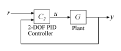
C2 = pidtune(G,'pidf2',1.5);C2 is a pid2 controller object. The control architecture for C2 is as shown in the following illustration.
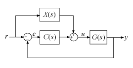
This control system can be equivalently represented in several other architectures that use only SISO components. In the feedforward configuration, the 2-DOF controller is represented as a SISO PID controller and a feedforward compensator.
Decompose C2 into SISO control components using the feedforward configuration.
[Cff,Xff] = getComponents(C2,'feedforward')Cff =
1 s
Kp + Ki * --- + Kd * --------
s Tf*s+1
with Kp = 1.12, Ki = 0.23, Kd = 1.3, Tf = 0.122
Continuous-time PIDF controller in parallel form.
Model Properties
Xff =
-10.898 (s+0.2838)
------------------
(s+8.181)
Continuous-time zero/pole/gain model.
Model Properties
This command returns the SISO PID controller Cff as a pid object. The feedforward compensator X is returned as a zpk object.
Construct the closed-loop system for the feedforward configuration.
Tff = G*(Cff+Xff)*feedback(1,G*Cff);
In the feedback configuration, the 2-DOF controller is represented as a SISO PID controller and an additional feedback compensator.
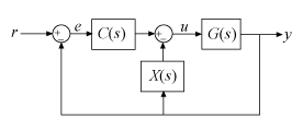
Decompose C2 using the feedback configuration and construct that closed-loop system.
[Cfb, Xfb] = getComponents(C2,'feedback');
Tfb = G*Cfb*feedback(1,G*(Cfb+Xfb));
In the filter configuration, the 2-DOF controller is represented as a SISO PID controller and prefilter on the reference signal.
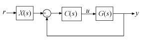
Decompose C2 using the filter configuration. Construct that closed-loop system as well.
[Cfr, Xfr] = getComponents(C2,'filter');
Tfr = Xfr*feedback(G*Cfr,1);
Construct the closed-loop system for the original 2-DOF controller, C2. To do so, convert C2 to a two-input, one-output transfer function, and use array indexing to access the channels.
Ctf = tf(C2);
Cr = Ctf(1);
Cy = Ctf(2);
T = Cr*feedback(G,Cy,+1);
Compare the step responses of all the closed-loop systems.
stepplot(T,Tff,Tfb,Tfr)
legend('2-DOF','feedforward','feedback','filter','Location','Southeast')
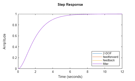
The plots coincide, demonstrating that all the systems are equivalent.
Using a 2-DOF PID controller can yield improved performance compared to a 1-DOF controller. For more information, see Tune 2-DOF PID Controller (Command Line).
See Also
pid2 | pidstd2 | getComponents