pid2
2-DOF PID controller in parallel form
Description
Use pid2 to create parallel-form, two-degree-of-freedom (2-DOF)
proportional-integral-derivative (PID) controller model objects, or to convert dynamic system models to parallel 2-DOF PID controller
form.
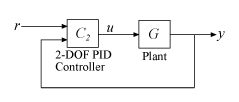
2-DOF PID controllers include setpoint weighting on the proportional and derivative terms. A 2-DOF PID controller can achieve fast disturbance rejection without significant increase of overshoot in setpoint tracking. 2-DOF PID controllers are also useful to mitigate the influence of changes in the reference signal on the control signal. The following illustration shows a typical control architecture using a 2-DOF PID controller.
The pid2 controller model object can represent parallel-form PID
controllers in continuous time or discrete time.
Continuous time —
Discrete time —
Here:
b is the setpoint weighting on the proportional term.
c is the setpoint weighting on the derivative term.
Kp is the proportional gain.
Ki is the integral gain.
Kd is the derivative gain.
Tf is the first-order derivative filter time constant.
IF(z) is the integrator method for computing the integral in the discrete-time controller.
DF(z) is the integrator method for computing the derivative filter in the discrete-time controller.
You can then combine this object with other components of a control architecture, such as the plant, actuators, and sensors to represent your control system. For more information, see Control System Modeling with Model Objects.
You can create a PID controller model object by either specifying the controller
parameters directly, or by converting a model of another type (such as a transfer function
model tf) to PID controller form.
You can also use pid2 to create generalized state-space (genss) models or uncertain state-space (uss (Robust Control Toolbox)) models.
Creation
You can obtain pid2 controller models in one of the following
ways.
Create a model using the
pid2function.Use the
pidtunefunction to tune PID controllers for a plant model. Specify a 2-DOF PID controller type in thetypeargument of thepidtunefunction to obtain a parallel-form 2-DOF PID controller. For example:sys = zpk([],[-1 -1 -1],1); C2 = pidtune(sys,'PID2');Interactively tune the PID controller for a plant model using:
The Tune PID Controller Live Editor task.
The PID Tuner app.
Syntax
Description
Input Arguments
Output Arguments
Properties
Object Functions
The following lists contain a representative subset of the functions you can use with pid2 models. In general, any function applicable to Dynamic System Models is applicable to a pid2 object.
Examples
Create a continuous-time 2-DOF controller with proportional and derivative gains and a filter on the derivative term. To do so, set the integral gain to zero. Set the other gains and the filter time constant to the desired values.
Kp = 1;
Ki = 0;   % No integrator
Kd = 3;
Tf = 0.1;
b = 0.5;    % setpoint weight on proportional term
c = 0.5;    % setpoint weight on derivative term
C2 = pid2(Kp,Ki,Kd,Tf,b,c)
C2 =

                         s
  u = Kp (b*r-y) + Kd -------- (c*r-y)
                       Tf*s+1

  with Kp = 1, Kd = 3, Tf = 0.1, b = 0.5, c = 0.5

Continuous-time 2-DOF PDF controller in parallel form.
Model Properties
The display shows the controller type, formula, and parameter values, and verifies that the controller has no integrator term.
Create a discrete-time 2-DOF PI controller using the trapezoidal discretization formula. Specify the formula using Name,Value syntax.
Kp = 5;
Ki = 2.4;
Kd = 0;
Tf = 0;
b = 0.5;
c = 0;
Ts = 0.1;
C2 = pid2(Kp,Ki,Kd,Tf,b,c,Ts,'IFormula','Trapezoidal')
C2 =

                      Ts*(z+1)
  u = Kp (b*r-y) + Ki -------- (r-y)
                      2*(z-1)

  with Kp = 5, Ki = 2.4, b = 0.5, Ts = 0.1

Sample time: 0.1 seconds
Discrete-time 2-DOF PI controller in parallel form.
Model Properties
Setting Kd = 0 specifies a PI controller with no derivative term. As the display shows, the values of Tf and c are not used in this controller. The display also shows that the trapezoidal formula is used for the integrator.
Create a 2-DOF PID controller, and set the dynamic system properties InputName and OutputName. Naming the inputs and the output is useful, for example, when you interconnect the PID controller with other dynamic system models using the connect command.
C2 = pid2(1,2,3,0,1,1,'InputName',{'r','y'},'OutputName','u')
C2 =

                       1
  u = Kp (b*r-y) + Ki --- (r-y) + Kd*s (c*r-y)
                       s

  with Kp = 1, Ki = 2, Kd = 3, b = 1, c = 1

Continuous-time 2-DOF PID controller in parallel form.
Model Properties
A 2-DOF PID controller has two inputs and one output. Therefore, the 'InputName' property is an array containing two names, one for each input. The model display does not show the input and output names for the PID controller, but you can examine the property values to see them. For instance, verify the input name of the controller.
C2.InputName
ans = 2×1 cell
    {'r'}
    {'y'}
Create a 2-by-3 grid of 2-DOF PI controllers with proportional gain ranging from 1–2 across the array rows and integral gain ranging from 5–9 across columns.
To build the array of PID controllers, start with arrays representing the gains.
Kp = [1 1 1;2 2 2];
Ki = [5:2:9;5:2:9];
When you pass these arrays to the pid2 command, the command returns the array of controllers.
pi_array = pid2(Kp,Ki,0,0,0.5,0,'Ts',0.1,'IFormula','BackwardEuler');
size(pi_array)
2x3 array of 2-DOF PID controller.
Each PID has 1 output and 2 inputs.
If you provide scalar values for some coefficients, pid2 automatically expands them and assigns the same value to all entries in the array. For instance, in this example, Kd = Tf = 0, so that all entries in the array are PI controllers. Also, all entries in the array have b = 0.5.
Access entries in the array using array indexing. For dynamic system arrays, the first two dimensions are the I/O dimensions of the model, and the remaining dimensions are the array dimensions. Therefore, the following command extracts the (2,3) entry in the array.
pi23 = pi_array(:,:,2,3)
pi23 =

                       Ts*z
  u = Kp (b*r-y) + Ki ------ (r-y)
                        z-1

  with Kp = 2, Ki = 9, b = 0.5, Ts = 0.1

Sample time: 0.1 seconds
Discrete-time 2-DOF PI controller in parallel form.
Model Properties
You can also build an array of PID controllers using the stack command.
C2 = pid2(1,5,0.1,0,0.5,0.5);         % PID controller
C2f = pid2(1,5,0.1,0.5,0.5,0.5);      % PID controller with filter
pid_array = stack(2,C2,C2f);          % stack along 2nd array dimension
These commands return a 1-by-2 array of controllers.
size(pid_array)
1x2 array of 2-DOF PID controller.
Each PID has 1 output and 2 inputs.
All PID controllers in an array must have the same sample time, discrete integrator formulas, and dynamic system properties such as InputName and OutputName.
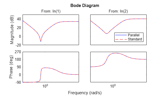
Convert a standard-form pidstd2 controller to parallel form.
Standard PID form expresses the controller actions in terms of an overall proportional gain Kp, integrator and derivative time constants Ti and Td, and filter divisor N. You can convert any 2-DOF standard-form controller to parallel form using the pid2 command. For example, consider the following standard-form controller.
Kp = 2;
Ti = 3;
Td = 4;
N = 50;
b = 0.1;
c = 0.5;
C2_std = pidstd2(Kp,Ti,Td,N,b,c)
C2_std =

                       1      1                      s
  u = Kp * [(b*r-y) + ---- * --- * (r-y) + Td * ------------ * (c*r-y)]
                       Ti     s                  (Td/N)*s+1

  with Kp = 2, Ti = 3, Td = 4, N = 50, b = 0.1, c = 0.5

Continuous-time 2-DOF PIDF controller in standard form
Convert this controller to parallel form using pid2.
C2_par = pid2(C2_std)
C2_par =

                       1                s
  u = Kp (b*r-y) + Ki --- (r-y) + Kd -------- (c*r-y)
                       s              Tf*s+1

  with Kp = 2, Ki = 0.667, Kd = 8, Tf = 0.08, b = 0.1, c = 0.5

Continuous-time 2-DOF PIDF controller in parallel form.
Model Properties
A response plot confirms that the two forms are equivalent.
bodeplot(C2_par,'b-',C2_std,'r--')
legend('Parallel','Standard','Location','Southeast')
Convert a discrete-time dynamic system that represents a 2-DOF PID controller with derivative filter to parallel pid2 form.
The following state-space matrices represent a discrete-time 2-DOF PID controller with a sample time of 0.1 s.
A = [1,0;0,0.99];
B = [0.1,-0.1; -0.005,0.01];
C = [3,0.2];
D = [2.6,-5.2];
Ts = 0.1;
sys = ss(A,B,C,D,Ts);
When you convert sys to 2-DOF PID form, the result depends on which discrete integrator formulas you specify for the conversion. For instance, use the default, ForwardEuler, for both the integrator and the derivative.
C2fe = pid2(sys)
C2fe =

                        Ts                   1
  u = Kp (b*r-y) + Ki ------ (r-y) + Kd ----------- (c*r-y)
                        z-1             Tf+Ts/(z-1)

  with Kp = 5, Ki = 3, Kd = 2, Tf = 10, b = 0.5, c = 0.5, Ts = 0.1

Sample time: 0.1 seconds
Discrete-time 2-DOF PIDF controller in parallel form.
Model Properties
Now convert using the Trapezoidal formula.
C2trap = pid2(sys,'IFormula','Trapezoidal','DFormula','Trapezoidal')
C2trap =

                      Ts*(z+1)                     1
  u = Kp (b*r-y) + Ki -------- (r-y) + Kd ------------------- (c*r-y)
                      2*(z-1)             Tf+Ts/2*(z+1)/(z-1)

  with Kp = 4.85, Ki = 3, Kd = 2, Tf = 9.95, b = 0.485, c = 0.5, Ts = 0.1

Sample time: 0.1 seconds
Discrete-time 2-DOF PIDF controller in parallel form.
Model Properties
The displays show the difference in resulting coefficient values and functional form.
Discretize a continuous-time 2-DOF PID controller and specify the integral and derivative filter formulas.
Create a continuous-time controller and discretize it using the zero-order-hold method of the c2d command.
C2con = pid2(10,5,3,0.5,1,1);  % continuous-time 2-DOF PIDF controller
C2dis1 = c2d(C2con,0.1,'zoh')
C2dis1 =

                        Ts                   1
  u = Kp (b*r-y) + Ki ------ (r-y) + Kd ----------- (c*r-y)
                        z-1             Tf+Ts/(z-1)

  with Kp = 10, Ki = 5, Kd = 3.31, Tf = 0.552, b = 1, c = 1, Ts = 0.1

Sample time: 0.1 seconds
Discrete-time 2-DOF PIDF controller in parallel form.
Model Properties
The display shows that c2d computes new PID coefficients for the discrete-time controller.
The discrete integrator formulas of the discretized controller depend on the c2d discretization method, as described in Tips. For the zoh method, both IFormula and DFormula are ForwardEuler.
C2dis1.IFormula
ans =
'ForwardEuler'
C2dis1.DFormula
ans =
'ForwardEuler'
If you want to use different formulas from the ones returned by c2d, then you can directly set the Ts, IFormula, and DFormula properties of the controller to the desired values.
C2dis2 = C2con;
C2dis2.Ts = 0.1;
C2dis2.IFormula = 'BackwardEuler';
C2dis2.DFormula = 'BackwardEuler';
However, these commands do not compute new PID gains for the discretized controller. To see this, examine C2dis2 and compare the coefficients to C2con and C2dis1.
C2dis2
C2dis2 =

                       Ts*z                   1
  u = Kp (b*r-y) + Ki ------ (r-y) + Kd ------------- (c*r-y)
                        z-1             Tf+Ts*z/(z-1)

  with Kp = 10, Ki = 5, Kd = 3, Tf = 0.5, b = 1, c = 1, Ts = 0.1

Sample time: 0.1 seconds
Discrete-time 2-DOF PIDF controller in parallel form.
Model Properties
Tips
To break a 2-DOF controller into two SISO control components, such as a feedback controller and a feedforward controller, use
getComponents.Create arrays of
pid2controller objects by:Specifying array values for one or more of the coefficients
Kp,Ki,Kd,Tf,b, andc.Specifying an array of dynamic systems
systo convert topid2controller objects.Using
stackto build arrays from individual controllers or smaller arrays.Passing an array of plant models to
pidtune.
In an array of
pid2controllers, each controller must have the same sample timeTsand discrete integrator formulasIFormulaandDFormula.To create or convert to a standard-form controller, use
pidstd2. Standard form expresses the controller actions in terms of an overall proportional gain Kp, integral and derivative times Ti and Td, and filter divisor N. For example, the relationship between the inputs and output of a continuous-time standard-form 2-DOF PID controller is given by:There are two ways to discretize a continuous-time
pid2controller:Use the
c2dcommand.c2dcomputes new parameter values for the discretized controller. The discrete integrator formulas of the discretized controller depend upon thec2ddiscretization method you use, as shown in the following table.c2dDiscretization MethodIFormulaDFormula'zoh'ForwardEulerForwardEuler'foh'TrapezoidalTrapezoidal'tustin'TrapezoidalTrapezoidal'impulse'ForwardEulerForwardEuler'matched'ForwardEulerForwardEulerFor more information about
c2ddiscretization methods, See thec2dreference page. For more information aboutIFormulaandDFormula, see Properties.If you require different discrete integrator formulas, you can discretize the controller by directly setting
Ts,IFormula, andDFormulato the desired values. (See Discretize a Continuous-Time 2-DOF PID Controller.) However, this method does not compute new gain and filter-constant values for the discretized controller. Therefore, this method might yield a poorer match between the continuous- and discrete-timepid2controllers than usingc2d.
Version History
Introduced in R2015b