bssm

Create Bayesian state-space model

Since R2022a

Description

bssm creates a bssm object, representing a Bayesian linear state-space model, from a specified parameter-to-matrix mapping function, which defines the state-space model structure, and the log prior distribution function of the parameters. The state-space model can be time-invariant or time-varying (see Decide on Model Structure), and the state or observation variables, x_t or y_t, respectively, can be multivariate series.

In general, a bssm object specifies the joint prior distribution and characteristics of the state-space model only. That is, the model object is a template intended for further use. Specifically, to incorporate data into the model for posterior distribution analysis, pass the model object and data to the appropriate object function.

Alternative state-space models include:

• The ssm model object — Standard linear Gaussian state-space model

• The dssm model object — Standard linear Gaussian state-space model with diffuse initial state distribution

• The bnlssm model object — Bayesian nonlinear non-Gaussian state-space model

Creation

Syntax

PriorMdl = bssm(ParamMap,ParamDistribution)

PriorMdl = bssm(ParamMap,ParamDistribution,Name=Value)

Description

There are several ways to create a bssm object representing a Bayesian state-space model:

• Create Prior Model — Directly create a bssm object, representing a prior model, by using the bssm function and specifying the parameter-to-matrix mapping function and log prior distribution function of the parameters. This method accommodates simple through complex state-space model structures. For more details, see the following syntax.

• Convert Standard Model to Bayesian Prior Model — Convert a specified standard, linear state-space model, an ssm object, to a bssm object by passing the model to the ssm2bssm function. The converted Bayesian model has the same state-space structure as the standard model. Use this method for simple state-space models when you prefer to specify the coefficient matrices explicitly. You can optionally specify the log prior density of the parameters. For details, see ssm2bssm and ssm.

• Estimate Posterior Model — Pass a bssm object representing a prior model, observed response data, and initial parameter values to the estimate function to obtain a bssm object representing a posterior model. For more details, see estimate.

PriorMdl = bssm(ParamMap,ParamDistribution) creates the Bayesian state-space model object PriorMdl, representing a prior model with Gaussian state disturbances and observation innovations, using the parameter-to-matrix mapping function ParamMap, which you write, and the log prior distribution of the parameters.

The ParamMap function maps the collection of linear state-space model parameters Θ to the time-invariant or time-varying coefficient matrices A, B, C, and D. In addition to the coefficient matrices, ParamMap can optionally map any of the following quantities:

• Initial state means and covariances Mean0 and Cov0

• State types StateType

• Deflated observation data DeflatedData to accommodate a regression component in the observation equation

The ParamDistribution function accepts Θ and returns the corresponding log density.

PriorMdl is a template that specifies the joint prior distribution of Θ and the structure of the state-space model.

PriorMdl = bssm(ParamMap,ParamDistribution,Name=Value) sets properties representing the distributions of the state disturbances and observation innovations using name-value arguments. For example, bssm(ParamMap,ParamDistribution,ObservationDistribution=struct("Name","t","DoF",6)) specifies t distribution with 6 degrees of freedom for all observation innovation variables u_t in the Bayesian state-space model.

Input Arguments

ParamMap — Parameter-to-matrix mapping function

function handle

Parameter-to-matrix mapping function that determines the data likelihood, specified as a function handle in the form @fcnName, where fcnName is the function name. ParamMap sets the ParamMap property. Object functions of bssm compute the data likelihood by using the standard Kalman filter, where probabilities additionally condition on the parameters.

Suppose paramMap is the name of the MATLAB^® function specifying how the state-space model parameters Θ map to the coefficient matrices and, optionally, other state-space model characteristics. Then, paramMap must have this form.

function [A,B,C,D,Mean0,Cov0,StateType,DeflateY] = paramMap(theta,...otherInputs...)
	...
end

where:

• theta is a numParams-by-1 numeric vector of the linear state-space model parameters Θ as the first input argument. The function can accept other inputs in subsequent positions.

• ParamMap returns the state-space model parameters in this table.

  Quantity	Output Position	Description
  At	1	Required state-transition coefficient matrix A
  Bt	2	Required state-disturbance-loading coefficient matrix B
  Ct	3	Required measurement-sensitivity coefficient matrix C
  Dt	4	Required observation-innovation coefficient matrix D
  μ0	5	Optional initial state mean vector Mean0
  Σ0	6	Optional initial state covariance matrix Cov0
  StateType	7	Optional state classification vector, either stationary (0), the constant 1 (1), or diffuse, static, or nonstationary (2)
  DeflatedData	8	Optional array of response data deflated by predictor data, which accommodates a regression component in the observation equation

  The subscript t indicates that the parameters can be time-varying (ignore the subscript for time-invariant parameters).

  To skip specifying an optional output argument, set the argument to [] in the function body. For example, to skip specifying Mean0, set Mean0 = []; in the function.

  For the default values of Mean0, Cov0, and StateType, see Algorithms.

Specify parameters to include in the posterior distribution by setting their value to an entry in the first input argument theta and set known entries of the coefficients to their values. For example, the following lines define the 1-D time-invariant state-space model

$$\begin{array}{l}{x}_t=a{x}_{t-1}+b{u}_t\\ y_t=x_t+d{\epsilon }_t.\end{array}$$

A = theta(1);
B = theta(2);
C = 1;
D = theta(3);

If paramMap requires the input parameter vector argument only, you can create the bssm object by calling:

Mdl = bssm(@paramMap,...)

In general, create the bssm object by calling:

Mdl = bssm(@(theta)paramMap(theta,...otherInputArgs...),...)

Example: bssm(@(params)paramFun(theta,y,z),@ParamDistribution) specifies the parameter-to-matrix mapping function paramFun that accepts the state-space model parameters theta, observed responses y, and predictor data z.

Tip

A best practice is to set StateType of each state within ParamMap for both of the following reasons:

• By default, the software generates StateType, but the default choice might not be accurate. For example, the software cannot distinguish between a constant 1 state and a static state.

• The software cannot infer StateType from data because the data theoretically comes from the observation equation. The realizations of the state equation are unobservable.

Data Types: function_handle

ParamDistribution — Log of joint probability density function of the state-space model parameters Π(Θ)

function handle

Log of joint probability density function of the state-space model parameters Π(Θ), specified as a function handle in the form @fcnName, where fcnName is the function name. ParamDistribution sets the ParamDistribution property.

Suppose logPrior is the name of the MATLAB function defining the joint prior distribution of Θ. Then, logPrior must have this form.

function logpdf = logPrior(theta,...otherInputs...)
	...
end

where:

• theta is a numParams-by-1 numeric vector of the linear state-space model parameters Θ. Elements of theta must correspond to those of ParamMap. The function can accept other inputs in subsequent positions.

• logpdf is a numeric scalar representing the log of the joint probability density of Θ at the input theta.

If ParamDistribution requires the input parameter vector argument only, you can create the bssm object by calling:

Mdl = bssm(...,@logPrior)

In general, create the bssm object by calling:

Mdl = bssm(...,@(theta)logPrior(theta,...otherInputArgs...))

Tip

Because out-of-bounds prior density evaluation is 0, set the log prior density of out-of-bounds parameter arguments to -Inf.

Data Types: function_handle

Properties

ParamMap — Parameter-to-matrix mapping function

function handle

Parameter-to-matrix mapping function, stored as a function handle and set by the ParamMap input argument. ParamMap completely specifies the structure of the state-space model.

Data Types: function_handle

ParamDistribution — Parameter distribution representation

function handle | numeric matrix

Parameter distribution representation, stored as a function handle or a numParams-by-numDraws numeric matrix.

• ParamDistribution is a function handle for the log prior distribution of the parameters ParamDistribution when you create PriorMdl directly by using bssm or when you convert a standard state-space model by using ssm2bssm.

• ParamDistribution is a numParams-by-numDraws numeric matrix containing random draws from the posterior distribution of the parameters when you estimate the posterior by using estimate. Rows correspond to the elements of theta and columns correspond to subsequent draws of the Markov chain Monte Carlo sampler, such as the Metropolis-Hastings sampler [1][2].

Data Types: function_handle

StateDistribution — Distribution of state disturbance process

"Gaussian" (default) | "t" | character vector | structure array

Since R2022b

Distribution of the state disturbance process, specified as a distribution name or structure array in this table. bssm stores the value as a structure array.

Distribution	Name	Variable Support	Structure Array	Hyperparameter Estimation Support
Standard Gaussian	"Gaussian"	Multivariate	struct("Name","Gaussian")	Not applicable
Student’s t	"t"	Multivariate	struct("Name","t","DoF",dof)	Yes

• The specified distribution applies to all state disturbance process variables.

• For the Student's t distribution:

  • If you supply a structure array, you must specify both the "Name" and "DoF" fields.

  • You can change the hyperparameter value by using dot notation after you create the model. For example, Mdl.Distribution.DoF = 3.

  • To facilitate posterior sampling, bssm represents multivariate Student's t-distributed variables as an inverse-gamma scale mixture. For more details, see Latent Variance Variables of t-Distributed Errors.

For more details on distribution hyperparameters, see Distribution Hyperparameters.

Example: struct("Name","t","DoF",6) specifies a t distribution with 6 degrees of freedom for the state disturbance process.

ObservationDistribution — Distribution of observation innovation process

"Gaussian" (default) | "t" | "mixture" | "Laplace" | "skewnormal" | character vector | structure array

Since R2022b

Distribution of the observation innovation process, specified as a distribution name or structure array in this table. bssm stores the value as a structure array.

Distribution	Name	Variable Support	Structure Array	Hyperparameter Estimation Support
Standard Gaussian	"Gaussian"	Multivariate	struct("Name","Gaussian")	Not applicable
Student’s t	"t"	Multivariate	struct("Name","t","DoF",dof)	Yes
Finite Gaussian mixture	"mixture"	Univariate	struct("Name","mixture","Weight",weight,"Mean",mu,"Variance",sigma2)	No
Laplace	"Laplace"	Univariate	struct("Name","Laplace")	Not applicable
Skew normal	"skewnormal"	Univariate	struct("Name","skewnormal","Delta",delta)	Yes

• The specified distribution applies to all observation innovation process variables. However, you can specify different Gaussian mixture regime means and variances among the variables.

• For the Student's t distribution:

  • If you supply a structure array, you must specify both the "Name" and "DoF" fields.

  • You can change the hyperparameter value by using dot notation after you create the model. For example, Mdl.Distribution.DoF = 3.

  • To facilitate posterior sampling, bssm represents multivariate Student's t-distributed variables as an inverse-gamma scale mixture. For more details, see Latent Variance Variables of t-Distributed Errors.

• For the finite Gaussian mixture distribution, bssm sets the number of regimes (mixture components) to the number of elements of weight. Therefore, to specify the nontrivial case, in which the distribution has more than one regime, you must specify at least weight.

For more details on distribution hyperparameters, see Distribution Hyperparameters.

Example: struct("Name","t","DoF",6) specifies a t distribution with 6 degrees of freedom for the state disturbance process.

Example: struct("Name","mixture","Mean",[-1 1],"Weight",[0.6 0.4]) specifies a two-regime Gaussian mixture model for the univariate observation innovation variable. The regime weights are 0.6 and 0.4. The regime mean vector is [-1 1]. The default variance for all regimes is 1.

Object Functions

estimate	Estimate posterior distribution of Bayesian state-space model parameters
simulate	Simulate posterior draws of Bayesian state-space model parameters
tune	Tune Bayesian state-space model posterior sampler

Examples

Create Time-Invariant Bayesian State-Space Model with Known and Unknown Parameters

Create a Bayesian state-space model containing two independent, stationary, autoregressive states. The observations are the deterministic sum of the two states (in other words, the model does not impose observation errors ${\epsilon }_{\mathit{t}}$). Symbolically, the system of equations is

$$\left[\begin{array}{c}{x}_{t,1}\\ x_{t,2}\end{array}\right]=\left[\begin{array}{cc}{\varphi }_1& 0\\ 0& {\varphi }_2\end{array}\right]\left[\begin{array}{c}{x}_{t-1,1}\\ x_{t-1,2}\end{array}\right]+\left[\begin{array}{cc}{\sigma }_1& 0\\ 0& {\sigma }_2\end{array}\right]\left[\begin{array}{c}{u}_{t,1}\\ u_{t,2}\end{array}\right]$$

$$y_t=\left[\begin{array}{cc}1& 1\end{array}\right]\left[\begin{array}{c}{x}_{t,1}\\ x_{t,2}\end{array}\right].$$

Arbitrarily assume that the prior distribution of ${\varphi }_1$, ${\varphi }_2$, ${\sigma }_1^2$, and ${\sigma }_2^2$ are independent Gaussian random variables with mean 0.5 and variance 1.

The Local Functions section contains two functions required to specify the Bayesian state-space model. You can use the functions only within this script.

The paramMap function accepts a vector of the unknown state-space model parameters and returns all of the following quantities:

• A = $\left[\begin{array}{cc}{\varphi }_1& 0\\ 0& {\varphi }_2\end{array}\right]$.

• B = $\left[\begin{array}{cc}{\sigma }_1& 0\\ 0& {\sigma }_2\end{array}\right]$.

• C = $\left[\begin{array}{cc}1& 1\end{array}\right]$.

• D = 0.

• Mean0 and Cov0 are empty arrays [], which specify the defaults.

• StateType = $\left[\begin{array}{cc}0& 0\end{array}\right]$, indicating that each state is stationary.

The paramDistribution function accepts the same vector of unknown parameters as does paramMap, but it returns the log prior density of the parameters at their current values. Specify that parameter values outside the parameter space have log prior density of -Inf.

Create the Bayesian state-space model by passing function handles directly to paramMap and paramDistribution to bssm.

Mdl = bssm(@paramMap,@priorDistribution)

Mdl = 
Mapping that defines a state-space model:
    @paramMap

Log density of parameter prior distribution:
    @priorDistribution

Mdl is a bssm model specifying the state-space model structure and prior distribution of the state-space model parameters. Because Mdl contains unknown values, it serves as a template for posterior estimation.

Local Functions

This example uses the following functions. paramMap is the parameter-to-matrix mapping function and priorDistribution is the log prior distribution of the parameters.

function [A,B,C,D,Mean0,Cov0,StateType] = paramMap(theta)
    A = [theta(1) 0; 0 theta(2)];
    B = [theta(3) 0; 0 theta(4)];
    C = [1 1];
    D = 0;
    Mean0 = [];         % MATLAB uses default initial state mean
    Cov0 = [];          % MATLAB uses initial state covariances
    StateType = [0; 0]; % Two stationary states
end

function logprior = priorDistribution(theta)
    paramconstraints = [(abs(theta(1)) >= 1) (abs(theta(2)) >= 1) ...
        (theta(3) < 0) (theta(4) < 0)];
    if(sum(paramconstraints))
        logprior = -Inf;
    else 
        mu0 = 0.5*ones(numel(theta),1); 
        sigma0 = 1;
        p = normpdf(theta,mu0,sigma0);
        logprior = sum(log(p));
    end
end

Create Time Varying Bayesian State-Space Model

Create a time-varying, Bayesian state-space model with these characteristics:

• From periods 1 through 250, the state equation includes stationary AR(2) and MA(1) models, respectively, and the observation model is the weighted sum of the two states.

• From periods 251 through 500, the state model includes only the first AR(2) model.

• ${\mu }_0=\left[\begin{array}{cccc}0.5& 0.5& 0& 0\end{array}\right]$ and ${\Sigma }_0$ is the identity matrix.

• The prior density is flat.

Symbolically, the state-space model is

$\begin{array}{l}\begin{array}{c}\left[\begin{array}{c}{x}_{1t}\\ x_{2t}\\ x_{3t}\\ x_{4t}\end{array}\right]=\left[\begin{array}{cccc}{\varphi }_1& {\varphi }_2& 0& 0\\ 1& 0& 0& 0\\ 0& 0& 0& \theta \\ 0& 0& 0& 0\end{array}\right]\left[\begin{array}{c}{x}_{1,t-1}\\ x_{2,t-1}\\ x_{3,t-1}\\ x_{4,t-1}\end{array}\right]+\left[\begin{array}{cc}{\sigma }_1& 0\\ 0& 0\\ 0& 1\\ 0& 1\end{array}\right]\left[\begin{array}{c}{u}_{1t}\\ u_{2t}\end{array}\right]\\ y_t=c_1\left(x_{1t}+x_{3t}\right)+{\sigma }_2{\epsilon }_t.\end{array}fort=1,...,250,\\ \begin{array}{c}\left[\begin{array}{c}{x}_{1t}\\ x_{2t}\end{array}\right]=\left[\begin{array}{cccc}{\varphi }_1& {\varphi }_2& 0& 0\\ 1& 0& 0& 0\end{array}\right]\left[\begin{array}{c}{x}_{1,t-1}\\ x_{2,t-1}\\ x_{3,t-1}\\ x_{4,t-1}\end{array}\right]+\left[\begin{array}{c}{\sigma }_1\\ 0\end{array}\right]u_{1t}\\ y_t=c_2{x}_{1t}+{\sigma }_3{\epsilon }_t.\end{array}fort=251,\\ \begin{array}{c}\left[\begin{array}{c}{x}_{1t}\\ x_{2t}\end{array}\right]=\left[\begin{array}{cc}{\varphi }_1& {\varphi }_2\\ 1& 0\end{array}\right]\left[\begin{array}{c}{x}_{1,t-1}\\ x_{2,t-1}\end{array}\right]+\left[\begin{array}{c}{\sigma }_1\\ 0\end{array}\right]u_{1t}\\ y_t=c_2{x}_{1t}+{\sigma }_3{\epsilon }_t.\end{array}fort=252,...,500.\end{array}$

Write a function that specifies how the parameters theta map to the state-space model matrices, the initial state moments, and the state types. Save this code as a file named timeVariantParamMap.m on your MATLAB® path. Alternatively, open the example to access the function.

function [A,B,C,D,Mean0,Cov0,StateType] = timeVariantParamMapBayes(theta,T)
% Time-variant, Bayesian state-space model parameter mapping function
% example. This function maps the vector params to the state-space matrices
% (A, B, C, and D), the initial state value and the initial state variance
% (Mean0 and Cov0), and the type of state (StateType). From periods 1
% through T/2, the state model is a stationary AR(2) and an MA(1) model,
% and the observation model is the weighted sum of the two states. From
% periods T/2 + 1 through T, the state model is the AR(2) model only. The
% log prior distribution enforces parameter constraints (see
% flatPriorBSSM.m).
    T1 = floor(T/2);
    T2 = T - T1 - 1;
    A1 = {[theta(1) theta(2) 0 0; 1 0 0 0; 0 0 0 theta(4); 0 0 0 0]};
    B1 = {[theta(3) 0; 0 0; 0 1; 0 1]}; 
    C1 = {theta(5)*[1 0 1 0]};
    D1 = {theta(6)};
    Mean0 = [0.5 0.5 0 0];
    Cov0 = eye(4);
    StateType = [0 0 0 0];
    A2 = {[theta(1) theta(2) 0 0; 1 0 0 0]};
    B2 = {[theta(3); 0]};
    A3 = {[theta(1) theta(2); 1 0]};
    B3 = {[theta(3); 0]}; 
    C3 = {theta(7)*[1 0]};
    D3 = {theta(8)};
    A = [repmat(A1,T1,1); A2; repmat(A3,T2,1)];
    B = [repmat(B1,T1,1); B2; repmat(B3,T2,1)];
    C = [repmat(C1,T1,1); repmat(C3,T2+1,1)];
    D = [repmat(D1,T1,1); repmat(D3,T2+1,1)];
end

Write a function that specifies a joint flat prior and parameter constraints. Save this code as a file named flatPriorBSSM.m on your MATLAB path. Alternatively, open the example to access the function.

function logprior = flatPriorBSSM(theta)
% flatPriorBSSM computes the log of the flat prior density for the eight
% variables in theta (see timeVariantParamMapBayes.m). Log probabilities
% for parameters outside the parameter space are -Inf.

    % theta(1) and theta(2) are lag 1 and lag 2 terms in a stationary AR(2)
    % model. The eigenvalues of the AR(1) representation need to be within
    % the unit circle.
    evalsAR2 = eig([theta(1) theta(2); 1 0]);
    evalsOutUC = sum(abs(evalsAR2) >= 1) > 0;

    % Standard deviations of disturbances and errors (theta(3), theta(6),
    % and theta(8)) need to be positive.
    nonnegsig1 = theta(3) <= 0;
    nonnegsig2 = theta(6) <= 0;
    nonnegsig3 = theta(8) <= 0;

    paramconstraints = [evalsOutUC nonnegsig1 ...
        nonnegsig2 nonnegsig3];
    if sum(paramconstraints) > 0
        logprior = -Inf;
    else
        logprior = 0;   % Prior density is proportional to 1 for all values
                        % in the parameter space.
    end
end

Create a bssm object representing the Bayesian state-space model object. Supply the parameter-to-matrix mapping function timeVariantParamMapBayes as a function handle of solely theta by setting the time series length to 500.

numObs = 500;
Mdl = bssm(@(theta)timeVariantParamMapBayes(theta,numObs),@flatPriorBSSM)

Mdl = 
Mapping that defines a state-space model:
    @(theta)timeVariantParamMapBayes(theta,numObs)

Log density of parameter prior distribution:
    @flatPriorBSSM

Specify t-Distributed State Disturbances

This example shows how to specify that the state disturbances of a Bayesian state-space model are Student's t distributed in order to model excess kurtosis in the state equation. The example shows how to prepare the degrees of freedom parameter for posterior estimation and the example fully specifies the distribution.

Consider the Bayesian state-space model in Create Time-Invariant Bayesian State-Space Model with Known and Unknown Parameters, but assume that the state disturbances are distributed as a Student's $\mathit{t}$ random variable.

Create the model by passing function handles to the local functions that represent the state-space model structure and prior distribution of the model parameters $\Theta$. Specify that the distribution of the state disturbances is Student's $\mathit{t}$.

Mdl = bssm(@paramMap,@priorDistribution,StateDistribution="t");
Mdl.StateDistribution

ans = struct with fields:
    Name: "t"
     DoF: NaN

Mdl is a bssm model. The property Mdl.StateDistribution is a structure array specifying the distribution of the state disturbances. The field DoF is NaN by default, which means that the $\mathit{t}$-distribution degrees of freedom ${\nu }_{\mathit{u}}$ is configured for estimation with all unknown state-space model parameters $\Theta$.

You can specify a fixed value for the degrees of freedom two ways:

• By setting the DoF field to the positive scalar using dot notation

• By recreating the bssm model and supplying a structure array specifying the distribution name and degrees of freedom

Specify that the degrees of freedom is 6 by using both methods.

Mdl.StateDistribution.DoF = 6

Mdl = 
Mapping that defines a state-space model:
    @paramMap

Log density of parameter prior distribution:
    @priorDistribution

Degree of freedom of t distribution in the state equation:
     6

statedist = struct("Name","t","DoF",6);
Mdl2 = bssm(@paramMap,@priorDistribution,StateDistribution=statedist)

Mdl2 = 
Mapping that defines a state-space model:
    @paramMap

Log density of parameter prior distribution:
    @priorDistribution

Degree of freedom of t distribution in the state equation:
     6

Mdl and Mdl2 are equal.

Local Functions

function [A,B,C,D,Mean0,Cov0,StateType] = paramMap(theta)
    A = [theta(1) 0; 0 theta(2)];
    B = [theta(3) 0; 0 theta(4)];
    C = [1 1];
    D = 0;
    Mean0 = [];         % MATLAB uses default initial state mean
    Cov0 = [];          % MATLAB uses initial state covariances
    StateType = [0; 0]; % Two stationary states
end

function logprior = priorDistribution(theta)
    paramconstraints = [(abs(theta(1)) >= 1) (abs(theta(2)) >= 1) ...
        (theta(3) < 0) (theta(4) < 0)];
    if(sum(paramconstraints))
        logprior = -Inf;
    else 
        mu0 = 0.5*ones(numel(theta),1); 
        sigma0 = 1;
        p = normpdf(theta,mu0,sigma0);
        logprior = sum(log(p));
    end
end

Specify Log Chi-Squared Distributed Observation Innovations

To model volatility clustering, you can specify $\log {\chi }_1^2$ distributed observation innovations by setting appropriate mixture weights, and regime means and variances of a 7-regime Gaussian mixture distribution.

Consider the Bayesian state-space model in Create Time-Invariant Bayesian State-Space Model with Known and Unknown Parameters, but assume that the observation-innovations process is distributed as a $\log {\chi }_1^2$ random variable.

Create a structure array with the following fields and values.

• Field Name with value "mixture"

• Field Weight with value [0.0089 0.0541 0.1338 0.2761 0.2923 0.1494 0.0854]

• Field Mean with value [-9.3202 -5.3145 -3.4147 -1.7097 -0.4531 0.3975 1.1925]

• Field Variance with value [3.2793 2.4574 1.8874 1.3121 0.8843 0.5898 0.4995].^2

weight = [0.0089 0.0541 0.1338 0.2761 0.2923 0.1494 0.0854];
mu = [-9.3202 -5.3145 -3.4147 -1.7097 -0.4531 0.3975 1.1925];
sigma2 = [3.2793 2.4574 1.8874 1.3121 0.8843 0.5898 0.4995].^2;

ObsInnovDist = struct("Name","mixture","Weight",weight, ...
    "Mean",mu,"Variance",sigma2);

Create the model by passing function handles to the local functions that represent the state-space model structure and prior distribution of the model parameters $\Theta$. Use the structure array ObsInnovDist to specify that the distribution of the observation innovations is finite Gaussian mixture with hyperparameters that define a $\log {\chi }_1^2$ distribution.

Mdl = bssm(@paramMap,@priorDistribution,ObservationDistribution=ObsInnovDist);
Mdl.ObservationDistribution

ans = struct with fields:
        Name: "mixture"
      Weight: [0.0089 0.0541 0.1338 0.2761 0.2923 0.1494 0.0854]
        Mean: [-9.3202 -5.3145 -3.4147 -1.7097 -0.4531 0.3975 1.1925]
    Variance: [10.7538 6.0388 3.5623 1.7216 0.7820 0.3479 0.2495]

Mdl is a bssm model. The property Mdl.ObservationDistribution is a structure array specifying the distribution of the observation-innovations process. All distribution hyperparameters are fully specified.

Plot the distribution of the observation innovations. Compare the Gaussian mixture representation of the $\log {\chi }_1^2$ and the true $\log {\chi }_1^2$ distributions.

r = numel(weight);
LogChi2GMMdl = gmdistribution(mu',reshape(sigma2,1,1,r),weight);
gmPDF = @(x)arrayfun(@(x0)pdf(LogChi2GMMdl,x0),x);
logchi2PDF = @(x)((1/sqrt(2*pi))*exp((x-exp(x))/2));
figure
fplot(gmPDF,[-10,5])
hold on
fplot(logchi2PDF,"--r")
title("Log Chi-Squared Distribution: Gaussian Mixture Versus True")
legend("Gaussian Mixture","True",Location="best")

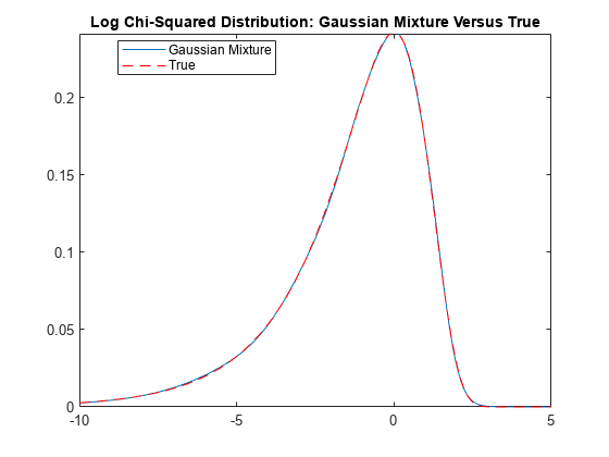
The distributions appear nearly identical.

Local Functions

function [A,B,C,D,Mean0,Cov0,StateType] = paramMap(theta)
    A = [theta(1) 0; 0 theta(2)];
    B = [theta(3) 0; 0 theta(4)];
    C = [1 1];
    D = 0;
    Mean0 = [];         % MATLAB uses default initial state mean
    Cov0 = [];          % MATLAB uses initial state covariances
    StateType = [0; 0]; % Two stationary states
end

function logprior = priorDistribution(theta)
    paramconstraints = [(abs(theta(1)) >= 1) (abs(theta(2)) >= 1) ...
        (theta(3) < 0) (theta(4) < 0)];
    if(sum(paramconstraints))
        logprior = -Inf;
    else 
        mu0 = 0.5*ones(numel(theta),1); 
        sigma0 = 1;
        p = normpdf(theta,mu0,sigma0);
        logprior = sum(log(p));
    end
end

Create Model Containing Regression Component to Deflate Observations

Consider a regression of the US unemployment rate onto and real gross national product (RGNP) rate, and suppose the resulting innovations are an ARMA(1,1) process. The state-space form of the relationship is

$$\begin{array}{l}\left[\begin{array}{c}{x}_{1,t}\\ x_{2,t}\end{array}\right]=\left[\begin{array}{cc}\varphi & \theta \\ 0& 0\end{array}\right]\left[\begin{array}{c}{x}_{1,t-1}\\ x_{2,t-1}\end{array}\right]+\left[\begin{array}{c}\sigma \\ 1\end{array}\right]u_t\\ y_t-\beta Z_t=x_{1,t},\end{array}$$

where:

• $$x_{1,t}$$ is the ARMA process.

• $$x_{2,t}$$ is a dummy state for the MA(1) effect.

• $$y_t$$ is the observed unemployment rate deflated by a constant and the RGNP rate ($$Z_t$$).

• $$u_t$$ is an iid Gaussian series with mean 0 and standard deviation 1.

Load the Nelson-Plosser data set, which contains a table DataTable that has the unemployment rate and RGNP series, among other series.

load Data_NelsonPlosser

Create a variable in DataTable that represents the returns of the raw RGNP series. Because price-to-returns conversion reduces the sample size by one, prepad the series with NaN.

DataTable.RGNPRate = [NaN; price2ret(DataTable.GNPR)];
T = height(DataTable);

Create variables for the regression. Represent the unemployment rate as the observation series and the constant and RGNP rate series as the deflation data ${\mathit{Z}}_{\mathit{t}}$.

Z = [ones(T,1) DataTable.RGNPRate];
y = DataTable.UR;

Write a function that specifies how the parameters theta map to the state-space model matrices, defers the initial state moments to the default, specifies the state types, and specifies the regression. Save this code as a file named armaDeflateYBayes.m on your MATLAB® path. Alternatively, open this example to access the function.

function [A,B,C,D,Mean0,Cov0,StateType,DeflatedY] = armaDeflateYBayes(theta,y,Z)
% Time-invariant, Bayesian state-space model parameter mapping function
% example. This function maps the vector parameters to the state-space
% matrices (A, B, C, and D), the default initial state value and the
% default initial state variance (Mean0 and Cov0), the type of state
% (StateType), and the deflated observations (DeflatedY). The log prior
% distribution enforces parameter constraints (see flatPriorDeflateY.m).
    A = [theta(1) theta(2); 0 0];
    B = [1; 1]; 
    C = [theta(3) 0];
    D = 0;
    Mean0 = [];
    Cov0 = [];
    StateType = [0 0];
    DeflatedY = y - Z*[theta(4); theta(5)];
end

Write a function that specifies a joint flat prior and parameter constraints. Save this code as a file named flatPriorDeflateY.m on your MATLAB path. Alternatively, open this example to access the function.

% Copyright 2022 The MathWorks, Inc.

function logprior = flatPriorDeflateY(theta)
% flatPriorDeflateY computes the log of the flat prior density for the five
% variables in theta (see armaDeflateYBayes.m). Log probabilities
% for parameters outside the parameter space are -Inf.

    % theta(1) and theta(2) are the AR and MA terms in a stationary
    % ARMA(1,1) model. The AR term must be within the unit circle.
    AROutUC = abs(theta(1)) >= 1;

    % The standard deviation of innovations (theta(3)) must be positive.
    nonnegsig1 = theta(3) <= 0;

    paramconstraints = [AROutUC nonnegsig1];
    if sum(paramconstraints) > 0
        logprior = -Inf;
    else
        logprior = 0;   % Prior density is proportional to 1 for all values
                        % in the parameter space.
    end
end

Create a bssm object representing the Bayesian state-space model. Specify the parameter-to-matrix mapping function as a handle to a function solely of the parameters theta.

Mdl = bssm(@(theta)armaDeflateYBayes(theta,y,Z),@flatPriorDeflateY)

Mdl = 
Mapping that defines a state-space model:
    @(theta)armaDeflateYBayes(theta,y,Z)

Log density of parameter prior distribution:
    @flatPriorDeflateY

More About

Bayesian Linear State-Space Model

A Bayesian linear state-space model is a Bayesian view of a standard linear state-space model, in which the vector of model parameters Θ are treated as random variables with a joint prior distribution Π(Θ) and a posterior distribution composed of the joint prior and data likelihood computed by the standard Kalman filter Π(Θ|y_t).

In general, a linear, multivariate, time-varying, Gaussian state-space model is the system of equations

$$\begin{array}{l}{x}_t=A_t{x}_{t-1}+B_t{u}_t\\ y_t-{\left(Z_t\beta \right)}^{\prime }=C_t{x}_t+D_t{\epsilon }_t,\end{array}$$

for t = 1, ..., T and where:

• $$x_t=\left[x_{1,t},\mathrm{...},x_{m_t,t}\right]\prime$$ is an m_t-dimensional state vector describing the dynamics of some, possibly unobservable, phenomenon at period t. The initial state distribution (x₀) has mean μ₀ (Mean0) and covariance matrix Σ₀ (Cov0).

• $$y_t=\left[y_{1,t},\mathrm{...},y_{n_t,t}\right]\prime$$ is an n_t-dimensional observation vector describing how the states are measured by observers at period t.

• $$u_t=\left[u_{1,t},\mathrm{...},u_{k_t,t}\right]\prime$$ is a k_t-dimensional white-noise vector of state disturbances at period t. All disturbances are either multivariate Gaussian distributed or multivariate Student's t distributed, with ν_u degrees of freedom.

• $${\epsilon }_t=\left[{\epsilon }_{1,t},\mathrm{...},{\epsilon }_{h_t,t}\right]\prime$$ is an h_t-dimensional white-noise vector of observation innovations at period t. All innovations are either multivariate Gaussian or Student's t distributed, or univariate finite Gaussian mixture, Laplace, or skew normal distributed.

• ε_t and u_t are uncorrelated.

• For time-invariant state-space models,

  • $$Z_t=\left[\begin{array}{cccc}{z}_{t1}& z_{t2}& \cdots & z_{td}\end{array}\right]$$ is row t of a T-by-d matrix of predictors Z. Each column of Z corresponds to a predictor, and each successive row to a successive period. If the observations are multivariate, then all predictors deflate each observation.

  • β is a d-by-n matrix of regression coefficients for Z_t.

• A_t, B_t, C_t, D_t, and β (when present) are model parameters arbitrarily collected in the vector Θ. The joint prior distribution of Θ is Π(Θ) and the joint posterior distribution of Θ is Π(Θ|y_t,Z_t).

The following definitions describe each of the model parameters and state characteristics, and how to configure them as outputs of ParamMap.

State-Transition Coefficient Matrix A_t

The state-transition coefficient matrix A_t is a matrix or cell vector of matrices that specifies how the states x_t are expected to transition from period t – 1 to t, for all t = 1,...,T. In other words, the expected state-transition equation at period t is E(x_t|x_t–1) = A_tx_t–1.

For time-invariant state-space models, the output A is an m-by-m matrix, where m is the number of state variables.

For time-varying state-space models, the output A is a series of matrices represented by a T-dimensional cell array, where A{t} contains an m_t-by-m_{t – 1} state-transition coefficient matrix. If the number of state variables changes from period t – 1 to t, m_t ≠ m_{t – 1}.

State-Disturbance-Loading Coefficient Matrix B_t

The state-disturbance-loading coefficient matrix B_t is a matrix or cell vector of matrices that specifies the additive error structure of the state disturbances u_t in the state-transition equation from period t – 1 to t, for all t = 1,...,T. In other words, the state-transition equation at period t is x_t = A_tx_t–1 + B_tu_t.

For time-invariant state-space models, the output B is an m-by-k matrix, where m is the number of state variables and k is the number of state disturbances. The quantity B*(B') is the state-disturbance covariance matrix for all periods.

For time-varying state-space models, B is a T-dimensional cell array, where B{t} contains an m_t-by-k_t state-disturbance-loading coefficient matrix. If the number of state variables or state disturbances changes at period t, the matrix dimensions between B{t-1} and B{t} vary. The quantity B{t}*(B{t}') is the state-disturbance covariance matrix for period t.

Measurement-Sensitivity Coefficient Matrix C_t

The measurement-sensitivity coefficient matrix C_t is a matrix or cell vector of matrices that specifies how the states x_t are expected to linearly combine at period t to form the observations, y_t, for all t = 1,...,T. In other words, the expected observation equation at period t is E(y_t|x_t) = C_tx_t.

For time-invariant state-space models, the output C is an n-by-m matrix, where n is the number of observation variables and m is the number of state variables.

For time-varying state-space models, the output C is a T-dimensional cell array, where C{t} contains an n_t-by-m_t measurement-sensitivity coefficient matrix. If the number of state or observation variables changes at period t, the matrix dimensions between C{t-1} and C{t} vary.

Observation-Innovation Coefficient Matrix D_t

The observation-innovation coefficient matrix D_t is a matrix or cell vector of matrices that specifies the additive error structure of the observation innovations ε_t in the observation equation at period t, for all t = 1,...,T. In other words, the observation equation at period t is y_t = C_tx_t + D_tε_t.

For time-invariant state-space models, the output D is an n-by-h matrix, where n is the number of observation variables and h is the number of observation innovations. The quantity D*(D') is the observation-innovation covariance matrix for all periods.

For time-varying state-space models, the output D is a T-dimensional cell array, where D{t} contains an n_t-by-h_t matrix. If the number of observation variables or observation innovations changes at period t, then the matrix dimensions between D{t-1} and D{t} vary. The quantity D{t}*(D{t}') is the observation-innovation covariance matrix for period t.

State Characteristics

Other state characteristics include initial state moments and a description of the dynamic behavior of each state.

You can optionally specify the state characteristics by including extra output arguments for ParamMap after the required coefficient matrices.

• Mean0 — Initial state mean μ₀, an m-by-1 numeric vector, where m is the number of states in x₁.

• Cov0 — Initial state covariance matrix Σ₀, an m-by-m positive semidefinite matrix.

• StateType — State dynamic behavior indicator, an m-by-1 numeric vector. This table summarizes the available types of initial state distributions.

  Value	State Dynamic Behavior Indicator
  0	Stationary (for example, ARMA models)
  1	The constant 1 (that is, the state is 1 with probability 1)
  2	Diffuse, nonstationary (for example, random walk model, seasonal linear time series), or static state

  For example, suppose that the state equation has two state variables: The first state variable is an AR(1) process, and the second state variable is a random walk. Specify the initial distribution types by setting StateType=[0; 2]; within the ParamMap function.

Static State

A static state does not change in value throughout the sample, that is, $$P\left(x_{t+1}=x_t\right)=1$$ for all t = 1,...,T.

Latent Variance Variables of t-Distributed Errors

To facilitate posterior sampling, multivariate Student's t-distributed state disturbances and observation innovations are each represented as an inverse-gamma scale mixture, where the inverse-gamma random variable is the latent variance variable.

Explicitly, suppose the m-dimensional state disturbances u_t are iid multivariate t distributed with location 0, scale I_m, and degrees of freedom ν_u. As an inverse-gamma scale mixture

$$u_t=\sqrt{{\zeta }_t}{\tilde{u}}_t,$$

where:

• The latent variable ζ_t is inverse-gamma with shape and scale ν_u/2.

• $${\tilde{u}}_t$$ is an m-dimensional multivariate standard Gaussian random variable.

Multivariate t-distributed observation innovations can be similarly decomposed.

You can access ζ_t by writing a custom output function that returns the field for the specified error type, either StateVariance or ObservationVariance. For more details, see the OutputFunction name-value argument and Output output argument.

Tips

• Load the data to the MATLAB workspace before creating the model.

• Create the parameter-to-matrix mapping function and log prior distribution function each as their own file.

• To specify a log χ²₁ distribution for the observation innovation process ε_t, set the ObservationDistribution to the structure array struct("Weight",weight,"Mean",mu,"Variance",sigma2), where:

  • weight is [0.0089 0.0541 0.1338 0.2761 0.2923 0.1494 0.0854].

  • mu is [-9.3202 -5.3145 -3.4147 -1.7097 -0.4531 0.3975 1.1925].

  • sigma2 is [3.2793 2.4574 1.8874 1.3121 0.8843 0.5898 0.4995].^2.

Algorithms

Distribution Hyperparameters

This table describes the supported distribution hyperparameters, and their values and defaults.

Distribution	Error Support	Hyperparameter	Field Name	Value	Default
Student's t	Multivariate ut (state) and εt (observation)	Degrees of freedom parameter	"DoF"	Positive numeric scalar, NaN, or a function handle. You must specify the value.	When you specify a structure array, you must specify "DoF". Otherwise, the default is NaN.
Finite Gaussian mixture	Univariate εt	Weights (probability distribution) for r regimes	"Weight"	Length r nonnegative vector. bssm normalizes the vector so that its elements sum to 1. bssm determines the number of regimes r by the number of elements of the value of "Weight".	1
		Means for r regimes	"Mean"	Length r finite numeric row vector	zeros(1,r)
		Variances for r regimes	"Variance"	Length r finite numeric row vector	ones(1,r)
Skew normal	Univariate εt	Distribution scale is $$\sqrt{{\delta }^2+1}$$ and shape is δ	"Delta"	Numeric scalar or NaN	NaN

• bssm fixes hyperparameters to specified numeric values.

• For a NaN or a function handle, where the values are supported, bssm treats the hyperparameter as unknown. Consequently, bssm object functions estimate them by computing their posterior distribution with all other unknown parameters in Θ. The value of the hyperparameter determines its prior distribution.

  • For NaN, the prior is flat.

  • For a function handle (supported for "DoF"), the associated function represents the log prior distribution. The function has the form, where x is a numeric scalar.

    function logpdf = logPrior(x,...otherInputs...)
    	...
    end

    For example, a valid function handle is @(x)log(normpdf(x,7,1)).

State-Space Model Behaviors

• For each state variable j, default values of Mean0 and Cov0 depend on StateType(j):

  • If StateType(j) = 0 (stationary state), bssm generates the initial value using the stationary distribution. If you provide all values in the coefficient matrices (that is, your model has no unknown parameters), bssm generates the initial values. Otherwise, the software generates the initial values during estimation.

  • If StateType(j) = 1 (constant state), Mean0(j) is 1 and Cov0(j) is 0.

  • If StateType(j) = 2 (nonstationary or diffuse state), Mean0(j) is 0 and Cov0(j) is 1e7.

• For static states that do not equal 1 throughout the sample, the software cannot assign a value to the degenerate, initial state distribution. Therefore, set the StateType of static states to 2. Consequently, the software treats static states as nonstationary and assigns the static state a diffuse initial distribution.

• bssm models do not store observed responses or predictor data. Supply the data wherever necessary using the appropriate input or name-value pair arguments.

• DeflateY is the deflated-observation data, which accommodates a regression component in the observation equation. For example, in this function, which has a linear regression component, Y is the vector of observed responses and Z is the vector of predictor data.

  function [A,B,C,D,Mean0,Cov0,StateType,DeflateY] = ParamFun(theta,Y,Z)
  	...
  	DeflateY = Y - params(9) - params(10)*Z;
  	...
  end

References

[1] Hastings, Wilfred K. "Monte Carlo Sampling Methods Using Markov Chains and Their Applications." Biometrika 57 (April 1970): 97–109. https://doi.org/10.1093/biomet/57.1.97.

[2] Metropolis, Nicholas, Rosenbluth, Arianna. W., Rosenbluth, Marshall. N., Teller, Augusta. H., and Teller, Edward. "Equation of State Calculations by Fast Computing Machines." The Journal of Chemical Physics 21 (June 1953): 1087–92. https://doi.org/10.1063/1.1699114.

Version History

Introduced in R2022a

R2022b: Assume non-Gaussian, fat-tailed distributions on the state disturbance and observation innovation processes

bssm enables you to assume the Student's t distribution for the conditional distribution of the state disturbance or observation innovations process. These error settings are suited when the process or measurement errors have excess kurtosis (or is fat-tailed or leptokuric).

Specify the distribution of either error process by using the following name-value argument when you create a bssm object:

• StateDistribution — Distribution of the state disturbance process

• ObservationDistribution — Distribution of the observation innovation process