plot

Visualize prior and posterior densities of Bayesian linear regression model parameters

Syntax

plot(PosteriorMdl)

plot(PriorMdl)

plot(PosteriorMdl,PriorMdl)

plot(___,Name,Value)

pointsUsed = plot(___)

[pointsUsed,posteriorDensity,priorDensity] = plot(___)

[pointsUsed,posteriorDensity,priorDensity,FigureHandle] = plot(___)

Description

plot(PosteriorMdl) or plot(PriorMdl) plots the posterior or prior distributions of the parameters in the Bayesian linear regression model PosteriorMdl or PriorMdl, respectively. plot adds subplots for each parameter to one figure and overwrites the same figure when you call plot multiple times.

plot(PosteriorMdl,PriorMdl) plots the posterior and prior distributions in the same subplot. plot uses solid blue lines for posterior densities and dashed red lines for prior densities.

plot(___,Name,Value) uses any of the input argument combinations in the previous syntaxes and additional options specified by one or more name-value pair arguments. For example, you can evaluate the posterior or prior density by supplying values of β and σ², or choose which parameter distributions to include in the figure.

pointsUsed = plot(___) also returns the values of the parameters that plot uses to evaluate the densities in the subplots.

[pointsUsed,posteriorDensity,priorDensity] = plot(___) also returns the values of the evaluated densities.

If you specify one model, then plot returns the density values in PosteriorDensity. Otherwise, plot returns the posterior density values in PosteriorDensity and the prior density values in PriorDensity.

[pointsUsed,posteriorDensity,priorDensity,FigureHandle] = plot(___) returns the figure handle of the figure containing the distributions.

Examples

Plot Prior and Posterior Distributions

Consider the multiple linear regression model that predicts the US real gross national product (GNPR) using a linear combination of industrial production index (IPI), total employment (E), and real wages (WR).

$${\text{GNPR}}_t={\beta }_0+{\beta }_1{\text{IPI}}_t+{\beta }_2{\text{E}}_t+{\beta }_3{\text{WR}}_t+{\epsilon }_t.$$

For all $$t$$, $${\epsilon }_t$$ is a series of independent Gaussian disturbances with a mean of 0 and variance $${\sigma }^2$$.

Assume these prior distributions:

• $$\beta |{\sigma }^2\sim N_4(M,{\sigma }^{2}V)$$. $$M$$ is a 4-by-1 vector of means, and $$V$$ is a scaled 4-by-4 positive definite covariance matrix.

• $${\sigma }^2\sim IG(A,B)$$. $$A$$ and $$B$$ are the shape and scale, respectively, of an inverse gamma distribution.

These assumptions and the data likelihood imply a normal-inverse-gamma conjugate model.

Create a normal-inverse-gamma conjugate prior model for the linear regression parameters. Specify the number of predictors p and the variable names.

p = 3;
VarNames = ["IPI" "E" "WR"];
PriorMdl = bayeslm(p,'ModelType','conjugate','VarNames',VarNames);

PriorMdl is a conjugateblm Bayesian linear regression model object representing the prior distribution of the regression coefficients and disturbance variance.

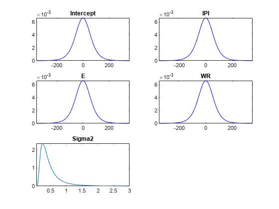
Plot the prior distributions.

plot(PriorMdl);

plot plots the marginal prior distributions of the intercept, regression coefficients, and disturbance variance.

Suppose that the mean of the regression coefficients is $$[-2040.0012{]}^{\prime }$$ and their scaled covariance matrix is

$$\left[\begin{array}{cccc}1& 0& 0& 0\\ 0& 0.001& 0& 0\\ 0& 0& 1e-8& 0\\ 0& 0& 0& 0.1\end{array}\right].$$

Also, the prior scale of the disturbance variance is 0.01. Specify the prior information using dot notation.

PriorMdl.Mu = [-20; 4; 0.001; 2];
PriorMdl.V = diag([1 0.001 1e-8 0.01]);
PriorMdl.B = 0.01;

Request a new figure and plot the prior distribution.

plot(PriorMdl);

plot replaces the current distribution figure with a plot of the prior distribution of the disturbance variance.

Load the Nelson-Plosser data set, and create variables for the predictor and response data.

load Data_NelsonPlosser
X = DataTable{:,PriorMdl.VarNames(2:end)};
y = DataTable.GNPR;

Estimate the posterior distributions.

PosteriorMdl = estimate(PriorMdl,X,y,'Display',false);

PosteriorMdl is a conjugateblm model object that contains the posterior distributions of $$\beta$$ and $${\sigma }^2$$.

Plot the posterior distributions.

plot(PosteriorMdl);

Plot the prior and posterior distributions of the parameters on the same subplots.

plot(PosteriorMdl,PriorMdl);

Plot Distributions to Separate Figures

Consider the regression model in Plot Prior and Posterior Distributions.

Load the Nelson-Plosser data set, create a default conjugate prior model, and then estimate the posterior using the first 75% of the data. Turn off the estimation display.

p = 3;
VarNames = ["IPI" "E" "WR"];
PriorMdl = bayeslm(p,'ModelType','conjugate','VarNames',VarNames);

load Data_NelsonPlosser
X = DataTable{:,PriorMdl.VarNames(2:end)};
y = DataTable.GNPR;

d = 0.75;
PosteriorMdlFirst = estimate(PriorMdl,X(1:floor(d*end),:),y(1:floor(d*end)),...
    'Display',false);

Plot the prior distribution and the posterior distribution of the disturbance variance. Return the figure handle.

[~,~,~,h] = plot(PosteriorMdlFirst,PriorMdl,'VarNames','Sigma2');

h is the figure handle for the distribution plot. If you change the tag name of the figure by changing the Tag property, then the next plot call places all new distribution plots on a different figure.

Change the name of the figure handle to FirstHalfData using dot notation.

h.Tag = 'FirstHalfData';

Estimate the posterior distribution using the rest of the data. Specify the posterior distribution based on the final 25% of the data as the prior distribution.

PosteriorMdl = estimate(PosteriorMdlFirst,X(ceil(d*end):end,:),...
    y(ceil(d*end):end),'Display',false);

Plot the posterior of the disturbance variance based on half of the data and all the data to a new figure.

plot(PosteriorMdl,PosteriorMdlFirst,'VarNames','Sigma2');

This type of plot shows the evolution of the posterior distribution when you incorporate new data.

Return Default Distribution and Evaluations

Consider the regression model in Plot Prior and Posterior Distributions.

Load the Nelson-Plosser data set and create a default conjugate prior model.

p = 3;
VarNames = ["IPI" "E" "WR"];
PriorMdl = bayeslm(p,'ModelType','conjugate','VarNames',VarNames);

load Data_NelsonPlosser
X = DataTable{:,PriorMdl.VarNames(2:end)};
y = DataTable.GNPR;

Plot the prior distributions. Request the values of the parameters used to create the plots and their respective densities.

[pointsUsedPrior,priorDensities1] = plot(PriorMdl);

pointsUsedPrior is a 5-by-1 cell array of 1-by-1000 numeric vectors representing the values of the parameters that plot uses to plot the corresponding densities. The first element corresponds to the intercept, the next three elements correspond to the regression coefficients, and the last element corresponds to the disturbance variance. priorDensities1 has the same dimensions as pointsUsed and contains the corresponding density values.

Estimate the posterior distribution. Turn off the estimation display.

PosteriorMdl = estimate(PriorMdl,X,y,'Display',false);

Plot the posterior distributions. Request the values of the parameters used to create the plots and their respective densities.

[pointsUsedPost,posteriorDensities1] = plot(PosteriorMdl);

pointsUsedPost and posteriorDensities1 have the same dimensions as pointsUsedPrior. The pointsUsedPost output can be different from pointsUsedPrior. posteriorDensities1 contains the posterior density values.

Plot the prior and posterior distributions. Request the values of the parameters used to create the plots and their respective densities.

[pointsUsedPP,posteriorDensities2,priorDensities2] = plot(PosteriorMdl,PriorMdl);

All output values have the same dimensions as pointsUsedPrior. The posteriorDensities2 output contains the posterior density values. The priorDensities2 output contains the prior density values.

Confirm that pointsUsedPP is equal to pointsUsedPost.

compare = @(a,b)sum(a == b) == numel(a);
cellfun(compare,pointsUsedPost,pointsUsedPP)

ans = 5×1 logical array

   1
   1
   1
   1
   1

The points used are equivalent.

Confirm that the posterior densities are the same, but that the prior densities are not.

cellfun(compare,posteriorDensities1,posteriorDensities2)

ans = 5×1 logical array

   1
   1
   1
   1
   1

cellfun(compare,priorDensities1,priorDensities2)

ans = 5×1 logical array

   0
   0
   0
   0
   0

When plotting only the prior distribution, plot evaluates the prior densities at points that produce a clear plot of the prior distribution. When plotting both a prior and posterior distribution, plot prefers to plot the posterior clearly. Therefore, plot can determine a different set of points to use.

Specify Values for Density Evaluation and Plotting

Consider the regression model in Plot Prior and Posterior Distributions.

Load the Nelson-Plosser data set and create a default conjugate prior model for the regression coefficients and disturbance variance. Then, estimate the posterior distribution and obtain the estimation summary table from summarize.

p = 3;
VarNames = ["IPI" "E" "WR"];
PriorMdl = bayeslm(p,'ModelType','conjugate','VarNames',VarNames);

load Data_NelsonPlosser
X = DataTable{:,PriorMdl.VarNames(2:end)};
y = DataTable.GNPR;

PosteriorMdl = estimate(PriorMdl,X,y);

Method: Analytic posterior distributions
Number of observations: 62
Number of predictors:   4
Log marginal likelihood: -259.348
 
           |   Mean      Std          CI95        Positive       Distribution      
-----------------------------------------------------------------------------------
 Intercept | -24.2494  8.7821  [-41.514, -6.985]    0.003   t (-24.25, 8.65^2, 68) 
 IPI       |   4.3913  0.1414   [ 4.113,  4.669]    1.000   t (4.39, 0.14^2, 68)   
 E         |   0.0011  0.0003   [ 0.000,  0.002]    1.000   t (0.00, 0.00^2, 68)   
 WR        |   2.4683  0.3490   [ 1.782,  3.154]    1.000   t (2.47, 0.34^2, 68)   
 Sigma2    |  44.1347  7.8020   [31.427, 61.855]    1.000   IG(34.00, 0.00069)     
 

summaryTbl = summarize(PosteriorMdl);
summaryTbl = summaryTbl.MarginalDistributions;

summaryTbl is a table containing the statistics that estimate displays at the command line.

For each parameter, determine a set of 50 evenly spaced values within three standard deviations of the mean. Put the values into the cells of a 5-by-1 cell vector following the order of the parameters that comprise the rows of the estimation summary table.

Points = cell(numel(summaryTbl.Mean),1); % Preallocation

for j = 1:numel(summaryTbl.Mean)
    Points{j} = linspace(summaryTbl.Mean(j) - 3*summaryTbl.Std(j),...
        summaryTbl.Mean(j) + 2*summaryTbl.Std(j),50);
end

Plot the posterior distributions within their respective intervals.

plot(PosteriorMdl,'Points',Points)

Input Arguments

PosteriorMdl — Bayesian linear regression model storing posterior distribution characteristics

conjugateblm model object | empiricalblm model object

Bayesian linear regression model storing posterior distribution characteristics, specified as a conjugateblm or empiricalblm model object returned by estimate.

When you also specify PriorMdl, then PosteriorMdl is the posterior distribution composed of PriorMdl and data. If the NumPredictors and VarNames properties of the two models are not equal, plot issues an error.

PriorMdl — Bayesian linear regression model storing prior distribution characteristics

conjugateblm model object | semiconjugateblm model object | diffuseblm model object | mixconjugateblm model object | lassoblm model object

Bayesian linear regression model storing prior distribution characteristics, specified as a conjugateblm, semiconjugateblm, diffuseblm, empiricalblm, customblm, mixconjugateblm, mixsemiconjugateblm, or lassoblm model object returned by bayeslm.

When you also specify PosteriorMdl, then PriorMdl is the prior distribution that, when combined with the data likelihood, forms PosteriorMdl. If the NumPredictors and VarNames properties of the two models are not equal, plot issues an error.

Name-Value Arguments

Specify optional pairs of arguments as Name1=Value1,...,NameN=ValueN, where Name is the argument name and Value is the corresponding value. Name-value arguments must appear after other arguments, but the order of the pairs does not matter.

Before R2021a, use commas to separate each name and value, and enclose Name in quotes.

Example: 'VarNames',["Beta1"; "Beta2"; "Sigma2"] plots the distributions of regression coefficients corresponding to the names Beta1 and Beta2 in the VarNames property of the model object and the disturbance variance Sigma2.

VarNames — Parameter names

cell vector of character vectors | string vector

Parameter names indicating which densities to plot in the figure, specified as the comma-separated pair consisting of 'VarNames' and a cell vector of character vectors or string vector. VarNames must include "Intercept", any name in the VarNames property of PriorMdl or PosteriorMdl, or "Sigma2".

By default, plot chooses "Intercept" (if an intercept exists in the model), all regression coefficients, and "Sigma2". If the model has more than 34 regression coefficients, then plot chooses the first through the 34th only.

VarNames is case insensitive.

Tip

If your model contains many variables, then try plotting subsets of the parameters on separate plots for a better view of the distributions.

Example: 'VarNames',["Beta(1)","Beta(2)"]

Data Types: string | cell

Points — Parameter values for density evaluation and plotting

numeric vector | cell vector of numeric vectors

Parameter values for density evaluation and plotting, specified as the comma-separated pair consisting of 'Points' and a numPoints-dimensional numeric vector or a numVarNames-dimensional cell vector of numeric vectors. numPoints is the number of parameters values that plot evaluates and plots the density.

• If Points is a numeric vector, then plot evaluates and plots the densities of all specified distributions by using its elements (see VarNames).

• If Points is a cell vector of numeric vectors, then:

  • numVarNames must be numel(VarNames), where VarNames is the value of VarNames.

  • Cells correspond to the elements of VarNames.

  • For j = 1,…,numVarNames, plot evaluates and plots the density of the parameter named VarNames{j} by using the vector of points in cell Points(j).

By default, plot determines 1000 adequate values at which to evaluate and plot the density for each parameter.

Example: 'Points',{1:0.1:10 10:0.2:25 1:0.01:2}

Data Types: double | cell

Output Arguments

pointsUsed — Parameter values used for density evaluation and plotting

cell vector of numeric vectors

Parameter values used for density evaluation and plotting, returned as a cell vector of numeric vectors.

Suppose Points and VarNames are the values of Points and VarNames, respectively. If Points is a numeric vector, then PointsUsed is repmat({Points},numel(VarNames)). Otherwise, PointsUsed equals Points. Cells correspond to the names in VarNames.

posteriorDensity — Evaluated and plotted posterior densities

cell vector of numeric row vectors

Evaluated and plotted posterior densities, returned as a numVarNames-by-1 cell vector of numeric row vectors. numVarNames is numel(VarNames), where VarNames is the value of VarNames. Cells correspond to the names in VarNames. posteriorDensity has the same dimensions as priorDensity.

priorDensity — Evaluated and plotted prior densities

cell vector of numeric row vectors

Evaluated and plotted prior densities, returned as a numVarNames-by-1 cell vector of numeric row vectors. priorDensity has the same dimensions as posteriorDensity.

FigureHandle — Figure window containing distributions

figure object

Figure window containing distributions, returned as a figure object.

plot overwrites the figure window that it produces.

If you rename FigureHandle for a new figure window, or call figure before calling plot, then plot continues to overwrite the current figure. To plot distributions to a different figure window, change the figure identifier of the current figure window by renaming its Tag property. For example, to rename the current figure window called FigureHandle to newFigure, at the command line, enter:

FigureHandle.Tag = newFigure;

Limitations

Because improper distributions (distributions with densities that do not integrate to 1) are not well defined, plot cannot plot them very well.

More About

Bayesian Linear Regression Model

A Bayesian linear regression model treats the parameters β and σ² in the multiple linear regression (MLR) model y_t = x_tβ + ε_t as random variables.

For times t = 1,...,T:

• y_t is the observed response.

• x_t is a 1-by-(p + 1) row vector of observed values of p predictors. To accommodate a model intercept, x_1t = 1 for all t.

• β is a (p + 1)-by-1 column vector of regression coefficients corresponding to the variables that compose the columns of x_t.

• ε_t is the random disturbance with a mean of zero and Cov(ε) = σ²I_T×T, while ε is a T-by-1 vector containing all disturbances. These assumptions imply that the data likelihood is

  $$\ell \left(\beta ,{\sigma }^2|y,x\right)={\displaystyle \prod _{t=1}^T\varphi \left(y_t;x_t\beta ,{\sigma }^2\right).}$$

  ϕ(y_t;x_tβ,σ²) is the Gaussian probability density with mean x_tβ and variance σ² evaluated at y_t;.

Before considering the data, you impose a joint prior distribution assumption on (β,σ²). In a Bayesian analysis, you update the distribution of the parameters by using information about the parameters obtained from the likelihood of the data. The result is the joint posterior distribution of (β,σ²) or the conditional posterior distributions of the parameters.

Version History

Introduced in R2017a