findstates

Estimate initial states of model

Syntax

x0 = findstates(sys,data)

x0 = findstates(sys,data,Horizon)

x0 = findstates(sys,data,Horizon,Options)

[x0,Report]= findstates(___)

Description

x0 = findstates(sys,data) estimates the initial states x0 of an identified model sys to maximize the fit between the model response and the output signal in the estimation data data. data can be a timetable, a comma-separated input/output matrix pair, or a time-domain or frequency-domain iddata object.

For timetables and data objects, findstates matches the input/output channels based on the channel names in sys and ignores nonmatching channels.

x0 = findstates(sys,data,Horizon) specifies the prediction horizon for computing the response of sys.

x0 = findstates(sys,data,Horizon,Options) specifies additional options for computation of x0.

[x0,Report]= findstates(___) delivers a report on the initial state estimation. Report is returned with any of the previous syntaxes.

Examples

Estimate Initial States of a Model

Create a nonlinear grey-box model. The model is a linear DC motor with one input (voltage), and two outputs (angular position and angular velocity). The structure of the model is specified by dcmotor_m.m file.

FileName = 'dcmotor_m'; 
Order = [2 1 2];
Parameters = [0.24365;0.24964];  
nlgr = idnlgrey(FileName,Order,Parameters);  
nlgr = setinit(nlgr, 'Fixed', false(2,1)); % set initial states free

Load data for initial state estimation.

load dcmotordata 
z = iddata(y,u,0.1);

Estimate the initial states such that the model's response using the estimated states X0 and measured input u is as close as possible to the measured output y.

X0 = findstates(nlgr,z,Inf);

Estimate Initial States of State-Space Model

Estimate an idss model and simulate it such that the response of the estimated model matches the estimation data's output signal as closely as possible.

Load sample data.

load iddata1 z1;

Estimate a linear model from the data.

model = ssest(z1,2);

Estimate the value of the initial states to best fit the measured output z1.y.

x0est = findstates(model,z1,Inf);

Simulate the model.

opt = simOptions('InitialCondition',x0est);
sim(model,z1(:,[],:),opt);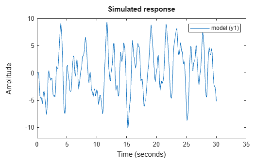

Selectively Estimate Initial States of a Model

Estimate the initial states of a model selectively by fixing the first state and allowing the second state of the model to be estimated.

Create a nonlinear grey-box model.

FileName = 'dcmotor_m'; 
Order = [2 1 2];
Parameters = [0.24365;0.24964];  
nlgr = idnlgrey(FileName,Order,Parameters);

The model is a linear DC motor with one input (voltage), and two outputs (angular position and angular velocity). The structure of the model is specified by dcmotor_m.m file.

Load the estimation data.

load dcmotordata
z = iddata(y,u,0.1);

Hold the first state fixed at zero, and estimate the value of the second.

x0spec = idpar('x0',[0;0]);
x0spec.Free(1) = false;
opt = findstatesOptions;
opt.InitialState = x0spec;
[X0,Report] = findstates(nlgr,z,Inf,opt)

X0 = 2×1

         0
    0.0061

Report = 
         Status: 'Estimated by simulation error minimization'
         Method: 'lsqnonlin'
     Covariance: [2x2 double]
       DataUsed: [1x1 struct]
    Termination: [1x1 struct]

Estimate Initial States by Specifying an Initial State Vector

Create a nonlinear grey-box model.

FileName = 'dcmotor_m'; 
Order = [2 1 2];
Parameters = [0.24365;0.24964];  
nlgr = idnlgrey(FileName,Order,Parameters);

The model is a linear DC motor with one input (voltage), and two outputs (angular position and angular velocity). The structure of the model is specified by dcmotor_m.m file.

Load the estimation data.

load dcmotordata
z = iddata(y,u,0.1);

Specify an initial guess for the initial states.

x0spec = idpar('x0',[10;10]);

x0spec.Free is true by default

Estimate the initial states

opt = findstatesOptions;
opt.InitialState = x0spec;
x0 = findstates(nlgr,z,Inf,opt)

x0 = 2×1

    0.0362
   -0.1322

Estimate Initial States Using Multi-Experiment Data

Create a nonlinear grey-box model.

FileName = 'dcmotor_m'; 
Order = [2 1 2];
Parameters = [0.24365;0.24964];  
nlgr = idnlgrey(FileName,Order,Parameters);  
set(nlgr, 'InputName','Voltage','OutputName', ...
		{'Angular position','Angular velocity'});

The model is a linear DC motor with one input (voltage), and two outputs (angular position and angular velocity). The structure of the model is specified by dcmotor_m.m file.

Load the estimation data.

load dcmotordata
z = iddata(y,u,0.1,'Name','DC-motor',...
     'InputName','Voltage','OutputName',...
     {'Angular position','Angular velocity'});

Create a three-experiment data set.

z3 = merge(z,z,z);

Choose experiment for estimating the initial states:

• Estimate initial state 1 for experiments 1 and 3

• Estimate initial state 2 for experiment 1

The fixed initial states have zero values.

x0spec = idpar('x0',zeros(2,3));
x0spec.Free(1,2) = false;
x0spec.Free(2,[2 3]) = false;
opt = findstatesOptions;
opt.InitialState = x0spec;

Estimate the initial states

[X0,EstInfo] = findstates(nlgr,z3,Inf,opt);

Input Arguments

sys — Identified model

idss object | idgrey object | idnlarx object | idnlhw object | idnlgrey object

Identified model whose initial states are estimated, represented as a linear state-space (idss or idgrey) or nonlinear model (idnlarx, idnlhw, or idnlgrey).

data — Estimation data

timetable | matrices | cell array | iddata object

Estimation data, specified as a uniformly sampled timetable, pair of input/output matrices, cell array, or iddata data object. The input/output dimensions of data must match sys. The specification for data depends on the data type.

Timetable

For SISO, MISO, and MIMO systems, specify data as a timetable that uses a regularly spaced time vector. For the timetable data type, data contains variables representing the input and output channels.

data must have the same variable names as the original data from which each model sys was estimated. The model properties include the names of the input and output variables. You therefore do not need to explicitly specify which channels to use in the timetable.

For multiexperiment data, specify data as a 1-by-Ne cell array, where Ne is the number of experiments. The sample times of all the experiments must match.

Matrices

For SISO, MISO, and MIMO systems, specify data as a pair of matrices with dimensions Ns-by-Nu for the input matrix and Ns-by-Ny for the output matrix. The software uses the sample period in the Ts property of sys.

For multiexperiment data, specify data as a pair of 1-by-Ne cell arrays, where Ne is the number of experiments. The sample times of all the experiments must match the sample time of sys.

iddata Object

For all model types, data can be a time-domain iddata object.

If sys is a linear model, data can also be a frequency-domain iddata object. For easier interpretation of initial conditions, make the frequency vector of data be symmetric about the origin. For converting time-domain data into frequency-domain data, use fft with the 'compl' input argument, and ensure that there is sufficient zero padding. Scale your data appropriately when you compare x0 between the time-domain and frequency-domain. Since for an N-point FFT, the input/output signals are scaled by 1/sqrt(N), the estimated x0 vector is also scaled by this factor.

For more information about working with estimation data types, see Data Domains and Data Types in System Identification Toolbox.

Horizon — Prediction horizon for computing model response

1 (default) | positive integer between 1 and Inf

Prediction horizon for computing the response of sys, specified as a positive integer between 1 and Inf. The most common values used are:

• Horizon = 1 — Minimizes the 1-step prediction error. The 1–step ahead prediction response of sys is compared to the output signals in data to determine x0. See predict for more information.

• Horizon = Inf — Minimizes the simulation error. The difference between measured output, data.y, and simulated response of sys to the measured input data, data.u is minimized. See sim for more information.

Specify Horizon as any positive integer between 1 and Inf, with the following restrictions:

Scenario	Horizon
Continuous-time model with time-domain data	1 or Inf
Continuous-time frequency-domain data (data.Ts = 0)	Inf
Output Error models (trivial noise component): Nonlinear grey-box (idnlgrey) Hammerstein-Wiener (idnlhw) Linear state-space with disturbance matrix, K = 0	Irrelevant Any value of Horizon returns the same answer for x0
Nonlinear ARX (idnlarx)	1 or Inf

Options — Estimation options for findstates

findstates Option set

Estimation options for findstates, specified as an option set created using findstatesOptions

Output Arguments

x0 — Estimated initial states

vector | matrix

Estimated initial states of model sys, returned as a vector or matrix. For multi-experiment data, x0 is a matrix with one column for each experiment.

Report — Initial state estimation information

structure

Initial state estimation information, returned as a structure. Report contains information about the data used, state covariance, and results of any numerical optimization performed to search for the initial states. Report has the following fields:

Report Field	Description
Status	Summary of how the initial state were estimated.
Method	Search method used.
Covariance	Covariance of state estimates, returned as a Ns-by-Ns matrix, where Ns is the number of states.
DataUsed	Attributes of the data used for estimation, returned as a structure with the following fields. Field Description Name Name of the data set. Type Data type. Length Number of data samples. Ts Sample time. InterSample Input intersample behavior, returned as one of the following values: 'zoh' — Zero-order hold maintains a piecewise-constant input signal between samples. 'foh' — First-order hold maintains a piecewise-linear input signal between samples. 'bl' — Band-limited behavior specifies that the continuous-time input signal has zero power above the Nyquist frequency. InputOffset Offset removed from time-domain input data during estimation. For nonlinear models, it is []. OutputOffset Offset removed from time-domain output data during estimation. For nonlinear models, it is [].
Termination	Termination conditions for the iterative search used for initial state estimation of nonlinear models. Structure with the following fields: Field Description WhyStop Reason for terminating the numerical search. Iterations Number of search iterations performed by the estimation algorithm. FirstOrderOptimality $$\infty$$-norm of the gradient search vector when the search algorithm terminates. FcnCount Number of times the objective function was called. UpdateNorm Norm of the gradient search vector in the last iteration. Omitted when the search method is 'lsqnonlin' or 'fmincon'. LastImprovement Criterion improvement in the last iteration, expressed as a percentage. Omitted when the search method is 'lsqnonlin' or 'fmincon'. Algorithm Algorithm used by 'lsqnonlin' or 'fmincon' search method. Omitted when other search methods are used. Termination is empty for linear models.

Version History

Introduced in R2015a

R2022b: Time-domain estimation data is accepted in the form of timetables and matrices

Most estimation, validation, analysis, and utility functions now accept time-domain input/output data in the form of a single timetable that contains both input and output data or a pair of matrices that contain the input and output data separately. These functions continue to accept iddata objects as a data source as well, for both time-domain and frequency-domain data.

R2018a: Advanced Options are deprecated for SearchOptions when SearchMethod is 'lsqnonlin'

Specification of lsqnonlin- related advanced options are deprecated, including the option to invoke parallel processing when estimating using the lsqnonlin search method, or solver, in Optimization Toolbox™.